By Valerio Cammelli
The remote detection of particulars electrical discharges of a thunderstorm allows us to determine the extent of the perturbation and its location if we implement techniques to determine the distance of discharges from the observation point. Observation networks are already active which, through a large number of receiving stations, provide a detailed map of the perturbation trend. These stations, which are connected to each other via the web, identify the longitude and latitude of the electric discharge through a triangulation process. The purpose of this work is to describe a method for detecting the distance of the discharge from the observation point by studying the characteristics of the radio signal generated by it. With this method it is possible to follow the trend of a distant perturbation (> 250 Km) using only one receiving station. Tweeks/sferics are electromagnetic perturbations caused by lightning of the type -CG + CG that propagate for reflections with the layer D or E for hundreds or thousands of Km. The band of the frequencies involved is the VLF-ELF. An example of sferic is that of fig.3, part of a series recorded in 2014.
SUMMARY OF THE PROPAGATION OF VLF
According to Wait's theory (1964) the propagation in the earth-ionosphere wave-guide is dispersive and the speed of the waves is a function of the frequency. The dynamic spectrum of the sferic shows an almost vertical line at highest frequencies and a curved line called " hook "at the lowest frequencies, which has an asymptotic value Fc (cut-off frequency), around 1700 Hz by night and which is determined by the height of the reflective layer.
The EM's propagation (ground-ionosphere) is characterized by the so-called modes which are: TM (transverse magnetic field), TE (transverse electric field), TEM (transverse electric and magnetic field).
Tweeks/sferic are generated by vertical lightning which excite TM and TEM modes. (Cummer 1997).
Short signals (1–10 ms) are typically recognized a sferics, tweek-atmospherics are electromagnetic pulses with duration of 10 – 100 ms.
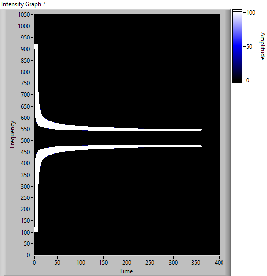
The highest modes TM2, TE2 and following, have an cut-off frequency Fc which is an integer multiple of the fundamental (see fig.7).
TEM mode is present for frequencies lower that Fc. Since the earth and the ionosphere are not perfect conductors the modes are not pure and they are defined qTM (quasi-TM).
We are interested only mode qTM1 which is the fundamental.
Note that these modes are strongly attenuated during the day, so the acquisition of tweeks/sferic is done during the night
DETAILS OF THE SIGNAL ACQUISITION
The signal is acquired by two perpendicular magnetic antennas ,they are made by 10 turns of 1.5 mmq wound on a square support of 1 m square. The pre-amplifier look like to the one described in ref. 6 by Marco Bruno, a double T notch analogue filter centred on 50 Hz was added because the environment is very noisy.
The analogue / digital conversion is performed by the 12-bit A-D converter USB-204 of Measurement Computing and SW Lab view 2015 of National Instruments. The sampling is at 48 KHz allowing a signal band of 24 KHz.The two channels N / S and E / are sampled for a total of 103,000 samples and a duration of acquisition about 2.1 sec.
DATA PROCESSING
For each channel there is a digital band-pass filter from 1000 Hz to 15000 Hz which reduces a lot the noise of 50 Hz and multiples up to the frequencies of interest of the tweeks/sferics (1400 Hz-15000 Hz).
To reduce more the noise of 50Hz and multiples it is necessary to use a lab-view function.This is "Extract Multiple Tone Information" , this function extracts all frequencies (tones) from the input signal, reconstructs a synthetic signal and subtracts it from the input signal. Figure 1 shows the input signal of the N / S channel.
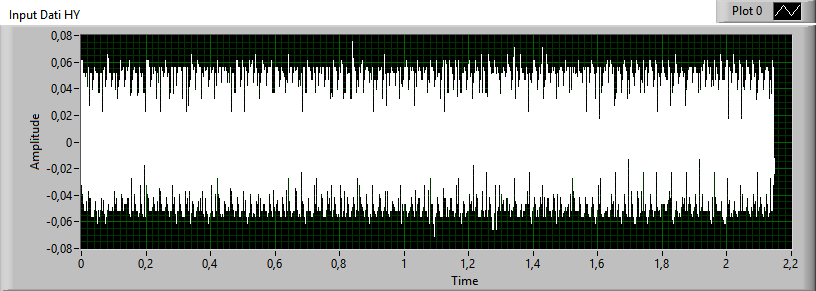
fig. 1
channel HY (N/S). Amplitude is in V, Time is in seconds.
The result of the application of the two filtrations is displayed in fig.2
A net improvement of the signal to noise ratio of about 12 dB is obtained.
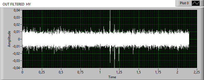
Fig.2
filtered input signal
The signal of fig.2 is sent to a the lab-view function: "Basic Mode Trigger Detection" by which an adjustable threshold can be set so the signal can pass only if it exceeds this value.
The operation is repeated for the E / O channel. It is considered a valid signal only if it exceeds a predetermined threshold on both channels. After that the trigger function also gives back the location of the trigger too respect to the origin of the acquisition.Then we can extract only the part which includes the tweek/sferic signal, if the maximum duration of the sferic has been set 8 ms. An example is shown in fig. 3.
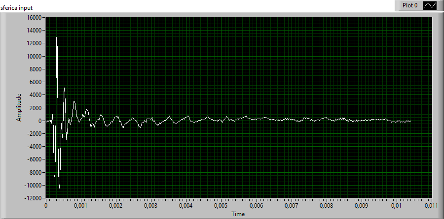
fig.3 : example of tweek
SPECTROGRAM OF THE SIGNAL
It is necessary to extract from the signal the necessary information for the characterization of the tweek/sferic parameters and this can be done only in the frequency-time domain.
One of the most important tools in the analysis of non-stationary signals is the STFT (Short Time Fourier Transform)
that can be thought as a Fourier transform or FFT (Fast Fourier Transform) applied to a rectangular window W(t). This window runs through the signal from its beginning to the end (see fig.4). The result is to have many spectra , each of them with its own spectral range.
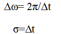
But we can not have simultaneous high discretization in frequency and time. In fact if we reduce the window size to have more temporal resolution we will have more uncertainty in the frequency.It can be shown the following relationship between time duration of a signal and the corresponding band in frequency: Δt x Δf ≥1 / 2.
The STFT is a complex quantity and its | STFT | ² magnitude represents the energy of the signal or spectrogram.
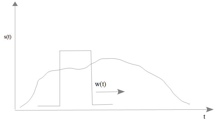
fig.4 Signal analisys with rectangular window
An evolution of
the STFT is the of GABOR TRANSFORM which can
be as an STFT with a W (t) gaussian window.
So we can be demonstrate that we reach
the maximum resolution both in
frequency than in time :
Δt. Δf = 1/2. (See the fig.5).
Δt. Δf = 1/2. (See the fig.5).
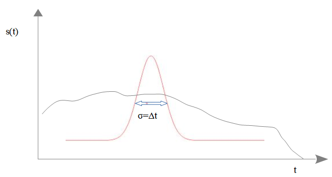
Fig.5 Gaussian window of the Gabor transform
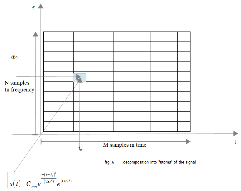
The signal in the frequency-time domain is computed into “atoms” consisting of complex coefficients Cmn multiplied by an elementary function:
Gaussian x sinusoid in the complex field.
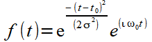 The Gabor
function can be considered as a Gaussian modulated in
frequency:
The Gabor
function can be considered as a Gaussian modulated in
frequency:exp - (t-tₒ) ² / 2σ² is the Gaussian window and
Since the signal is sampled with interval Δ t we can express
and
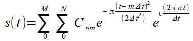
this is the Gabor expansion of the signal or Gabor inverse transform.
As the transform : Cm,n =
expresses the complex coefficients and therefore the magnitude and phase of the Gabor transform. Here γ (t) is the dual function of the gabor function and is also called analysis window, N is the number of samples in frequency (512). The number of samples during the time (M) has been set at 400, (spheric average length 8 ms).
The Lab-view sw with the "time frequency analysis" tool provides the function: "TFA fast Gabor Spectrogram" which is used to represent the signal energy distribution, useful for determining whether a tweek/sferic is to be processed or not.
The figure 7 shows the Gabor spectrogram of the same sferic/tweek :
The displayed frequency is limited to 10 KHz which are sufficient for the representation.
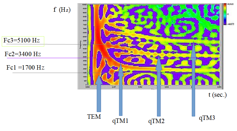
Fig.7 Gabor Spectrogram
For the single
mode the theoretical curve in the frequency-time
domain of the sferic only depends on the
frequency of cut-off Fc and the distance
from the source d , according to the following
formula (Yano et al 1989):
(1)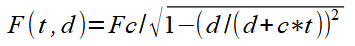
In this case c is the speed of light, t is the time from the beginning of the sferic signal.
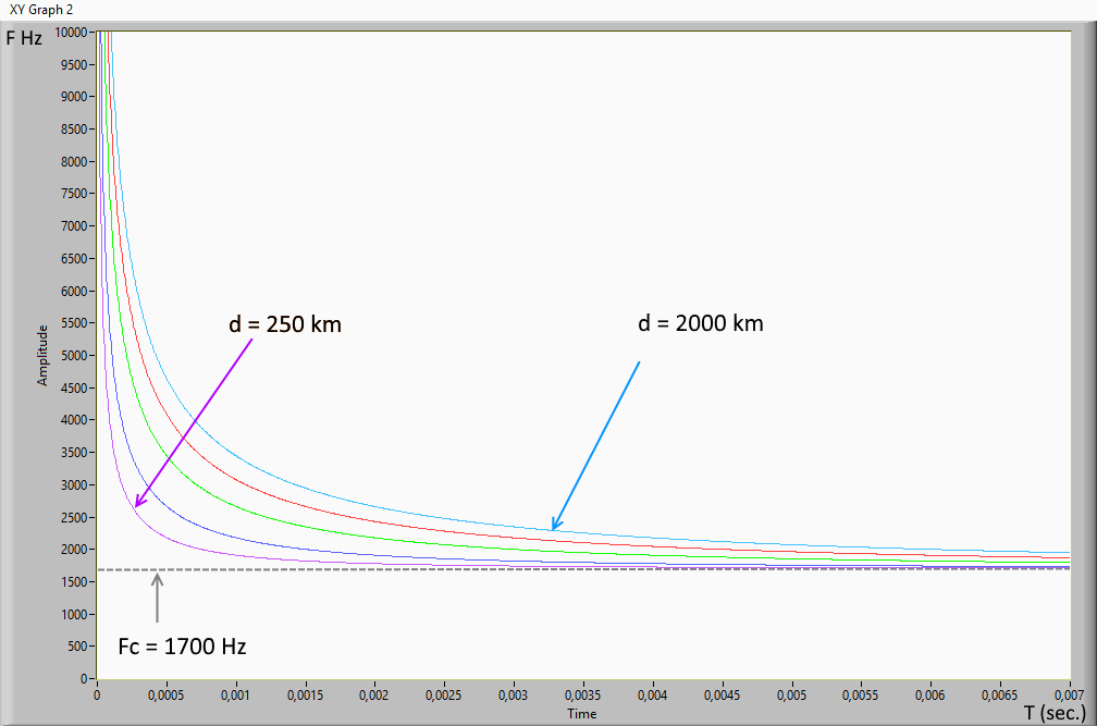
Fig. 8 Graph of (1)
The figure 8 shows the graph of the previous formula when d changes, ( the distance from the source is in meters with cut-off frequency Fc = 1700 Hz average value). The cut-off frequency can changes by night in the 1500-2400 Hz range.
Possibles methods to calculate the distance of the tweek
1. If you look to fig. 8 and fig.7 you can see immediately a method to estimate the distance of the sferic :
Put the transparent graph xy of fig. 8 upon on fig. 7 ; before you have equalized the dimensions and the scales in x and y of the two graphs.At last we choose the curve of fig.8 which best fits the shape of the sferic on the spectrogram.The method works but is manual and limited by the discretization of the curves in fig.8.
2. Timing Varying filter
I suppose to separate the qTM1 mode from the other modes in the frequency- time domain. So we would have a filtered signal in the time domain which unlike the sferic of fig.1,would consists of quasi-sinusoids of decreasing frequencies up to Fc. We could so easily to apply at this signal an algorithm to derive the instantaneous frequency as a function of time and then to match these points with the theoretical curve (1) and so obtain d .
Unfortunately we can not use the Gabor spectrogram because it is not invertible.
To separate the components of a frequency-time representation, the Gabor transform is performed first,
the representation is modified by masking the zone of interest and then the inverse-transform is applied to obtain the filtered signal.
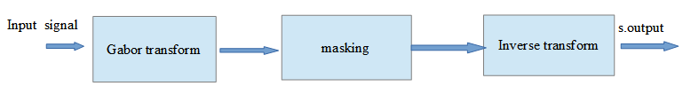
The sw Lab-view 2015 with the "time frequency analysis" tool-kit has all the functions related to the Gabor transform and inverse transform , but to create a mask it is also necessary to work with the images with the "Vision lab-view " package and to develop a special program.
1) Gabor transform of the sferic signal of fig. 3
We use the lab-view function "TFA discrete Gabor Transform" which creates an array of complex numbers :
The magnitude represents the Gabor transform of the tweek/sferic signal of fig. 3.
As we see in fig. 9 the transform produces less details of the spectrogram of fig. 7 because the spectrogram is a representation of the energy of the signal. The frequency in ordinates is limited to 10.000 Hz, in abscissa the time is in second.
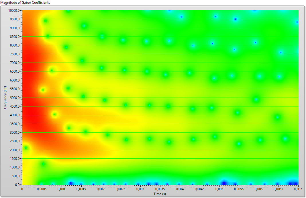
fig.9 Array magnitude Gabor transform M = 400 N = 512
2) Masking
The output of the Gabor transform function is an xy array of complex numbers, for our purposes we obtain its magnitude which is shown in fig.9.The discretization in frequency is 24KHz / 512 = 46.875 Hz and the
the sampling interval is 1 / 48KHz.= 20,833 μs.
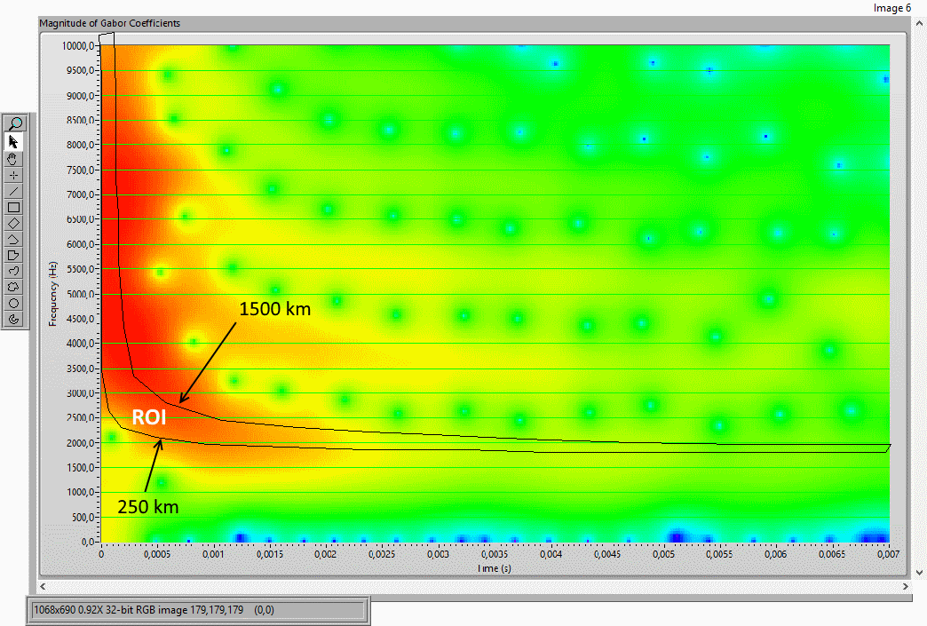
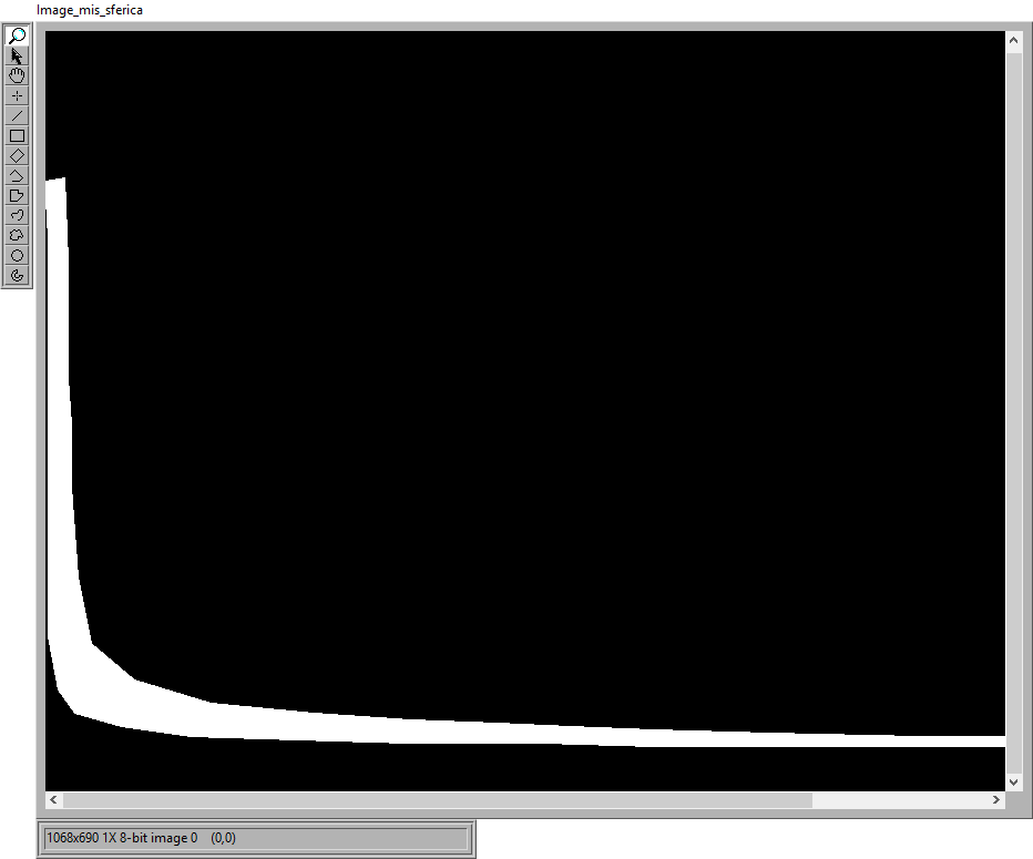
Using a Lab-View function (Vision) we obtain the RGB image of the same array on which you can manually draw an ROI (Region Of Interest) bounded by the curve d = 250 Km and to the curve d = 1500 Km of fig.8 with the horizontal part of the curve d = 250 Km at the Fc = 1700 Hz At this point another function transforms the ROI in a black-white image (mask) see fig.11.
The black /white image of the mask of fig.11 is transformed into an array. But, since the Gabor coefficients include also the negative frequencies, a symmetric mask must be built for the negative frequencies. The two arrays must be joined (fig.12).
The obtained array size is 1024 x 400 as the size of the array of Gabor transform magnitude of signal.
3) filtered signal
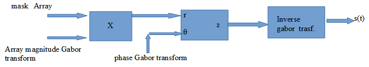
fig. 13
fig.13 shows the sequence of operations to obtain the filtered signal: the mask array of fig.12 is multiplied by the array magnitude of Gabor transform in fig. 9: Only the white regions of the mask will let the magnitude array but it is now necessary to add the phase obtained from the Gabor transform to obtain the complex array to which the inverse-transformation of Gabor is applied, the result is a signal in the time purified of all the upper and lower modes (Fig. 14).
4) calculation of the instantaneous frequency of the filtered signal
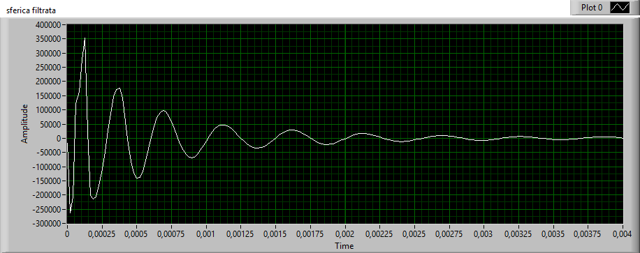
The GZC algorithm (Generalized Zero Crossing) is used but it is not available as a Lab-view function, so it must be implemented (fig.15) by developing a specific program.
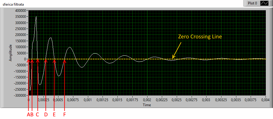
Fig.15 - filtered tweek
Called a, b, c, d ... the points of the zero crossing of the signal and Ta, Tb, Tc, Td ....
the respective times interval from the origin, we calculate the first frequency Fa = 1 / Tc-Ta , considered at the medium time Tb, the second frequency Fb = 1 / Td-Tb , considered at the time Tc, the third frequency Fc = 1 / Te- Tc, considered at the time Td and so on, the various frequencies and relative times can therefore be drawn in an XY chart, the result is a series of points in the frequency time domain that approximate a sferic of the type shown in fig.8.
5) Data fitting and distance calculation
To calculate the distance d we must identify which curve among those that are described by eq. (1)
better approximate the data.
We will use the function of the lab-view math library: "non linear curve fit LM”
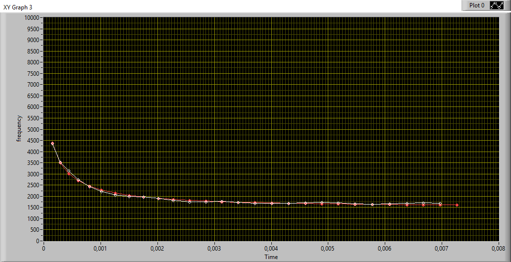
In fig.16 (graph xy) the points obtained from the GZC algorithm are shown in white. The "best fit" points corresponding to the parameter d which in the equation (1) approximates the data, are shown in red.
The function directly gives the value of the distance that in our case is 1009 Km with variance 143.
We must explain another important parameter of the sferic that must be obtained independently: the cut-off frequency Fc that typically takes the value 1700 Hz overnight but that can changes between 1500 Hz and 2500 Hz.
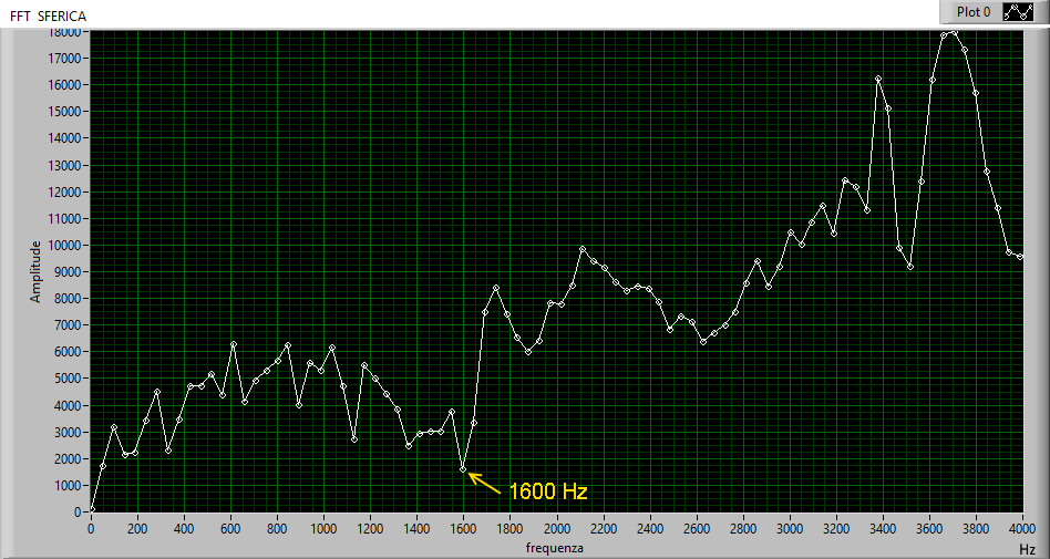
Fig.17 magnitude FFT of tweek di fig.3
(1)
In this case c is the speed of light, t is the time from the beginning of the sferic signal.
Fig. 8 Graph of (1)
The figure 8 shows the graph of the previous formula when d changes, ( the distance from the source is in meters with cut-off frequency Fc = 1700 Hz average value). The cut-off frequency can changes by night in the 1500-2400 Hz range.
Possibles methods to calculate the distance of the tweek
1. If you look to fig. 8 and fig.7 you can see immediately a method to estimate the distance of the sferic :
Put the transparent graph xy of fig. 8 upon on fig. 7 ; before you have equalized the dimensions and the scales in x and y of the two graphs.At last we choose the curve of fig.8 which best fits the shape of the sferic on the spectrogram.The method works but is manual and limited by the discretization of the curves in fig.8.
2. Timing Varying filter
I suppose to separate the qTM1 mode from the other modes in the frequency- time domain. So we would have a filtered signal in the time domain which unlike the sferic of fig.1,would consists of quasi-sinusoids of decreasing frequencies up to Fc. We could so easily to apply at this signal an algorithm to derive the instantaneous frequency as a function of time and then to match these points with the theoretical curve (1) and so obtain d .
Unfortunately we can not use the Gabor spectrogram because it is not invertible.
To separate the components of a frequency-time representation, the Gabor transform is performed first,
the representation is modified by masking the zone of interest and then the inverse-transform is applied to obtain the filtered signal.
The sw Lab-view 2015 with the "time frequency analysis" tool-kit has all the functions related to the Gabor transform and inverse transform , but to create a mask it is also necessary to work with the images with the "Vision lab-view " package and to develop a special program.
1) Gabor transform of the sferic signal of fig. 3
We use the lab-view function "TFA discrete Gabor Transform" which creates an array of complex numbers :
The magnitude represents the Gabor transform of the tweek/sferic signal of fig. 3.
As we see in fig. 9 the transform produces less details of the spectrogram of fig. 7 because the spectrogram is a representation of the energy of the signal. The frequency in ordinates is limited to 10.000 Hz, in abscissa the time is in second.
fig.9 Array magnitude Gabor transform M = 400 N = 512
2) Masking
fig.10
image of array and ROI
The output of the Gabor transform function is an xy array of complex numbers, for our purposes we obtain its magnitude which is shown in fig.9.The discretization in frequency is 24KHz / 512 = 46.875 Hz and the
the sampling interval is 1 / 48KHz.= 20,833 μs.
Using a Lab-View function (Vision) we obtain the RGB image of the same array on which you can manually draw an ROI (Region Of Interest) bounded by the curve d = 250 Km and to the curve d = 1500 Km of fig.8 with the horizontal part of the curve d = 250 Km at the Fc = 1700 Hz At this point another function transforms the ROI in a black-white image (mask) see fig.11.
 |
 |
|
fig.11 white / black mask
image |
fig.12 array mask
|
The black /white image of the mask of fig.11 is transformed into an array. But, since the Gabor coefficients include also the negative frequencies, a symmetric mask must be built for the negative frequencies. The two arrays must be joined (fig.12).
The obtained array size is 1024 x 400 as the size of the array of Gabor transform magnitude of signal.
3) filtered signal
fig. 13
fig.13 shows the sequence of operations to obtain the filtered signal: the mask array of fig.12 is multiplied by the array magnitude of Gabor transform in fig. 9: Only the white regions of the mask will let the magnitude array but it is now necessary to add the phase obtained from the Gabor transform to obtain the complex array to which the inverse-transformation of Gabor is applied, the result is a signal in the time purified of all the upper and lower modes (Fig. 14).
fig.
14 filtered sferic
4) calculation of the instantaneous frequency of the filtered signal
The GZC algorithm (Generalized Zero Crossing) is used but it is not available as a Lab-view function, so it must be implemented (fig.15) by developing a specific program.
Fig.15 - filtered tweek
Called a, b, c, d ... the points of the zero crossing of the signal and Ta, Tb, Tc, Td ....
the respective times interval from the origin, we calculate the first frequency Fa = 1 / Tc-Ta , considered at the medium time Tb, the second frequency Fb = 1 / Td-Tb , considered at the time Tc, the third frequency Fc = 1 / Te- Tc, considered at the time Td and so on, the various frequencies and relative times can therefore be drawn in an XY chart, the result is a series of points in the frequency time domain that approximate a sferic of the type shown in fig.8.
5) Data fitting and distance calculation
To calculate the distance d we must identify which curve among those that are described by eq. (1)
better approximate the data.
We will use the function of the lab-view math library: "non linear curve fit LM”
fig. 16 data fitting with formula
(1)
distance km = 1009,04
variance = 143.513
In fig.16 (graph xy) the points obtained from the GZC algorithm are shown in white. The "best fit" points corresponding to the parameter d which in the equation (1) approximates the data, are shown in red.
The function directly gives the value of the distance that in our case is 1009 Km with variance 143.
We must explain another important parameter of the sferic that must be obtained independently: the cut-off frequency Fc that typically takes the value 1700 Hz overnight but that can changes between 1500 Hz and 2500 Hz.
Fig.17 magnitude FFT of tweek di fig.3
The Fc is
obtained by carrying out the FFT of the sferic
signal considering only its magnitude as shown
in fig.17.
The first linear rise of the amplitude represented on the abscissa is the Fc, which can be obtained automatically developing a special algorithm.
The value of the Fc is also used to center the mask on the sferic by using an image shift function of “vision” to move the mask vertically so that the qTM1 mode is at the center of the mask.
CONCLUSIONS
The records were obtained on the outskirts of Florence, in an area with high E.M. pollution. For this reason the acquisition system has been equipped with both analog and digital filters to reduce the 50 Hz and its harmonics.
Some recordings have been compared with data from the Blitzortung.org network which calculates the positions of lightning trough the triangulation of different receiving stations. The error found by the exposed method is about 10% if the tweeks/sferics are clearly discernible in the spectrogram by shape and intensity.
Bibliography
1. “ Theory of communication “ D. Gabor J. IEE, vol. 93, pp. 429–457, 1946.
2. “Ionospheric D region remote sensing using VLF radio atmospheric” S. A. Cummer U. S. Inan and T. F. Bell Radio Science, 33, 1781–1792, November–December 1998
3. “Development of an automatic procedure to estimate the reflection height of tweek atmospherics”
Hiroyo Ohya1, Kazuo Shiokawa2, and Yoshizumi Miyoshi2 Earth Planets Space, 60, 837–843, 2008
4. Yano, S. Wave-form analysis of tweek atmospherics [Text] / S. Yano, T. Ogawa, H. Hagino // Res. Lett. Atmos. Electr. – 1989. – 9. – P. 31-42.
5. James R. Wait. Electromagnetic Waves in Stratified Media. Pergamon
Press, 1962. Reprinted 1996, IEEE Press.
6. “Thinking about ideal loop” Marco Bruno , Radio Waves below 22 Khz , Feb.2001.