The interest of Renato (and mine as
well) was to try to establish a method for detecting the direction of arrival
(DOA) of each signal recorded with this antenna. Renato describes in his
web page a method (effective but a bit cumbersome) to process the recorded
data with Cooledit. My goal (not very different from Renato's ideas, as
I discovered!) was to setup a DSP method that could perform a sort of real-time
DOA analysis.
The idea I wanted to implement was
pretty close to the Watson-Watt
RDF method: in this method two antennas with orthogonal radiation patterns
pick-up the unknown signal. The antennas are connected to two receivers,
whose output are sent (after some integration) to the x- and y- channels
of a scope. The incoming signal plots on the screen a line whose azimut
is equal to the DOA, apart an ambiguity of +/- 180 degrees.
To remove the ambiguity a third omnidirectional
antenna is used to blank the unwanted part of the signal on the scope.
The drawback of the method is the need for three receivers, that must have
pretty well matched phases and gains. The Watson Watt method was modified
by multiplexing the signals into one receiver, moving the complexity of
the technique from the receiver set to the antenna system.
Now back to our data: since the dataset
I received had only two channels of data (coming from the two crossed loops),
I expected of course that I could not get rid of the 180 degrees ambiguity.
There was also a further ambiguity, due to the fact that I had no idea
about how the loops were connected to the sound card! I guessed I could
work blindly, and then estimate the antenna directions given the azimuths
obtained for some known signals. During the experiments more ideas came
to my mind about how to implement the method, but first I wanted to implement
a straight version of the Watson Watt device, of course using DSP methods....
|
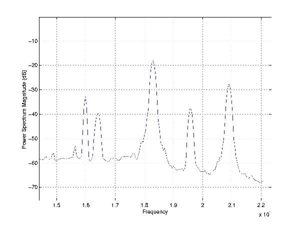
Let us call the two channels I had as channel "A" and channel "B". Each channel consisted of 2295608 samples, and the sampling rate was of 44100 Hz. I began selecting some frequencies to analyze, namely GBR at 16.0 kHz, HWU at 18.3 and 20.9 kHz and I could not resist go give a glance also to the ubiquitous 50 Hz... Here you can see part of the power spectrum on the "A" channel. |
The processing
method
The processing method applied to
the
signals was very straightforward: channels A and B were filtered with a
costant-Q FIR bandpass filter (Q = 100, FIR length = 121 taps), and for
each pair of samples I plotted a point on a x-y graph: I expected that
the incoming direction could show up as a straight line. In parallel I
also computed the direction of arrival fitting a least-square line to the
signals, i.e. B = mA + q where B and A are our signals, and m and
q are the parameters fitted to the data. The parameter q takes into account
the fact that we expect that our "receiver" could have a DC bias, while
from m we can compute the direction of arrival, since DOA = atan(m).
The results
obtained
Here we can see the results obtained:
| Station | Estimated DOA | Graph |
| GBR 16 kHz | 37.6 degrees | 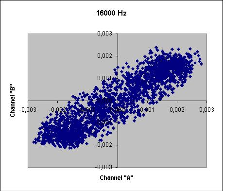 |
| HWU 18.3 kHz | 59.1 degrees | 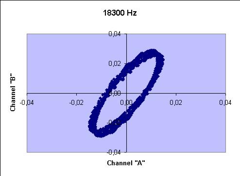 |
| HWU 20.9 kHz | 37.7 degrees | 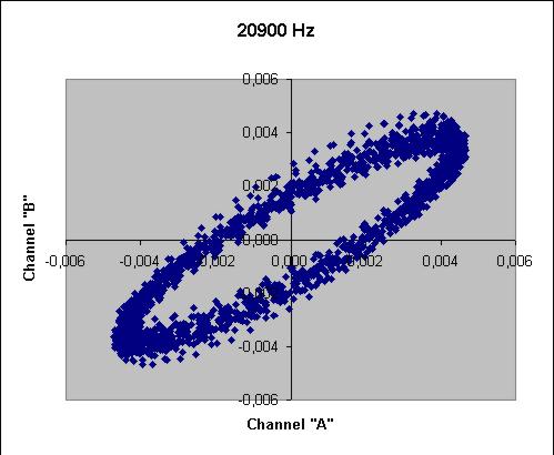 |
| ENEL 50 Hz | ? ! ? | 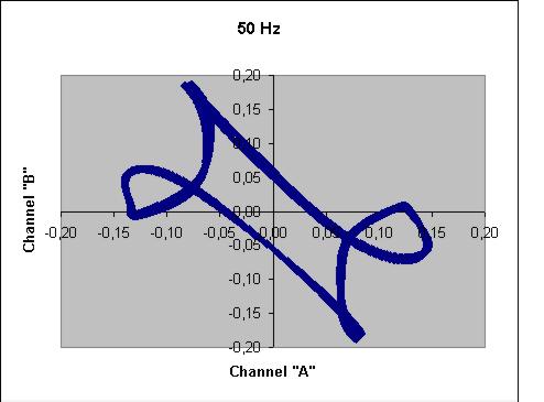 |
As you can see, the result are quite confusing....let us try to understand something from our data!
At first, the analysis of the signal at 50 Hz shows us that the "pest" noise does not have a preferred DOA. This is a bad news if one hopes to reduce it by properly directing a loop antenna. The traces on the X-Y plot are very sharp, thanks to the very high SNR ratio of this guy....
The signal from HWU draws a strange elliptical pattern. I guess it is modulated in RTTY, so it is tempting to assume that different tones show different DOA, but I cannot yet understand the reason. I'll have to analyze more carefully the data to check this...
Results comparison
| And now let's give a look at what I measured, what Renato found with his method, and the true DOA. The parenteses in the second column simply add 90 degrees to the measurement, since I did not know the correct orientation of the "A' and "B" channels. |
|
I do not know if the dataset received by me was also analyzed by Renato with his method, and if he could repeat the measurements he has shown in his web page.
What I can see is that:
Next it comes to explain the large (30 degrees !) error in the measurement of HWU (18.3). The signal is quite strong, and as it can be seen from the X-Y graph, the traces are quite sharp. I wonder if Renato measured the same dataset he sent me. Maybe we have to make some further tests to improve my result. As soon as I can set up a orking method, we could think about a way to make the method more "user friendly"...
I also tried a FFT-based DOA analysis:
it was the same method described above, computed in the frequency domain.
Results were very disappointing, and they are not shown here. I will come
back to the FFT method as soon as I can properly detect the DOA of HWU
and maybe GBR.
Next steps could be: