Many years have passed since a radioamateurs'
s ability only was in his ear. The home computer diffusion and the
very many software free distributions made possible for everyone the DSP
function. That is Digital Signal Processing. Spectrogram, FFT and
Frequency Resolution became famous words of frequent use, even
if these functions and the upcoming data are difficult to read.
In this article we'll try to explain these words,
and by doing it we'll se what link there is between them. We think,
this is a basic think to learn and to know for who approaches the natural
origin radio signal study. So, the description will be not so much scientific
and mathematics but more pragmatic. Only basic formulas will be given,
those which will find their practical application in the natural and not
natural origin radio signal study.
A radio signal demodulated from our receiver, or
simply gotten by a vlf receiver without conversion, consists on an electric
signal changing during the time. This is the easiest way to represent a
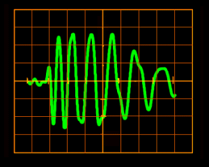
signal, that is the time representation: what we can visualize on the oscilloscope
screen in analogical pattern.
|
|
|
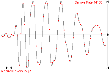
| A signal represented in a time domain, on the oscilloscope screen. | The same signal, as represented and archived in a wave file, like a points of values sequence |
| SAMPLES:
1210
BITSPERSAMPLE: 16 SAMPLERATE: 22050 1352 1027 689 1135 1 1335 1010 999 590 563 -113 -382 -357 .... |
In the audio card of our computer the
signal goes from an analogical pattern to a digital one, becoming a long
number list which are the same signal. The signal is taken
with regular time intervals and a value measuring is done:
by doing this we'll have very important data. What does this operation
is called A/D converter. Our signal is now in a digital form. A wave file
simply is the reading of this measuring.
We can imagine a wave file like a number series
after an header were are reported samples number, bit and sample rate
|
These valuing gives the max represented frequency
following the formulae:
|
Fmax = Sample Rate / 2 |
The Fmax value is often called "Nyquist Frequency".
If for instance we take a signal 11025 SR/SEC we
have a band which goes from 0 to 5512,5 Hz.
FOURIER FFT AND SIGNAL SPECTRUM
G. B. Fourier was a mathematics who lived between
1700 and 1800: he showed that any function which changes in time can be
divided in single periodic signals.
Applied on an electric signal: any signal of a
certain lasting which changes in a random way in time can be divided
in single frequencies which represent it, obtaining so a representation
of the frequency domain.
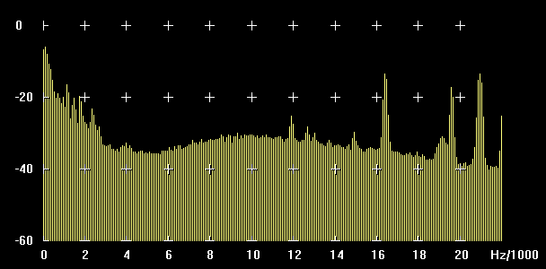 |
SPECTRUM
In picture there is the spectrum in frequency of the signal, the one we know, commonly as FFT that is a bar system indicating the signal level by single frequency and that change constantly. |
|
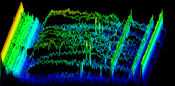 |
3D SPECTROGRAM
Different spectrum in succession, which give the representation of how the spectrum changes frequency with the time, are called spectrograms. This kind of representation, called 3D spectrogram is very choreographic but not as much representative. |
|
 |
2D SPECTROGRAM
The most common way to represent on of them, by associate colors (mostly gray) to intensity signals, is the classic spectrogram one, also called waterfall display. |
FFT NUMBERS
The speech, as concept is very simple, but as soon
as we approach the factors which control the FFT, we understand that the
representation can be done in a very many ways.
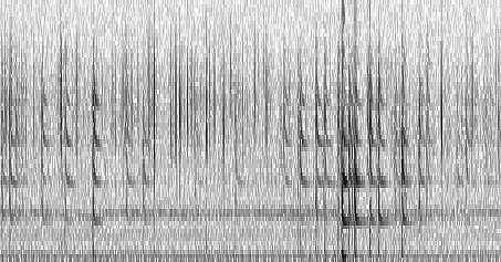 |
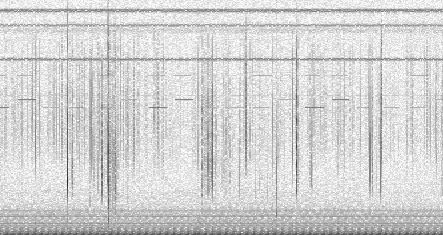
First example:
3 seconds 0-11 kHz frequency range FFT 64 points |
|
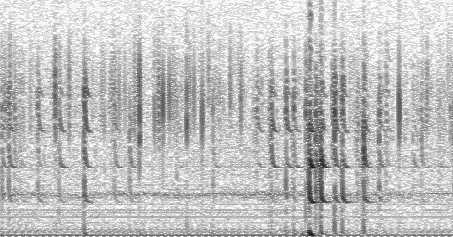 |
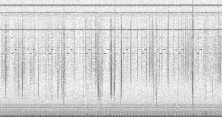
Second example:
3 seconds 0-11 kHz frequency range FFT 256 points |
|
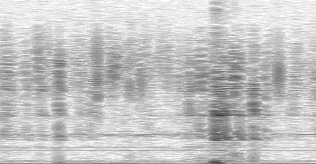 |
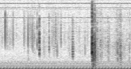
Third example:
3 seconds 0-11 kHz frequency range FFT 1024 points |
The three spectrograms show the same wave file represented in the same way: 3 sec, 0-11 KHz frequency range.
Looking at the pictures we can see that by changing
the FFT points number, the image loses definition in frequency or in the
time.
Let's see way:
The FFT calculation is based on a certain amount
of points which can be chosen during the analysis.
The FFT number can be also called Buffer FFT.
The value of Buffer FFT gives the amount of yellow bars which appear in
the graphic (The picture above called SPECTRUM) following the formulae:
|
Spectrum Bars = FFT Buffer / 2 |
For instance: a FFT of 1024 PTS gives a representation of 512 bars.
The number of FFT points also gives
the frequency resolution, that is how many Hz are represented by
a single bar (that is how large the every single bar band filter is). An
FFT bar is also called "FFT bin" in literature to emphasize that it contains
the energy (or effective voltage) from a frequency range, not a single
frequency (english: "bin" ~ bucket, container; german: "Eimer", italian:
bidone).
You can see it this way: For SR=44100 Hz, a frequency
range of 22050 Hz is equally split into 512 bins (or "bars"), every
bin is 22050 / 512 = 43.066 Hz wide.
The leftmost bin, this is the one containing the
lowest frequency, has only half the width of all other bins. From the example
above, the 1st bin covers 0.000 Hz ... 21.5 Hz.
|
Frequency Resolution = Sample Rate / FFT Points = Frequency range / Bins numbers |
For instance with a SR of 44100 sample/sec and 1024 FFT points we have a frequency resolution of 44 Hz.
The number of points gives the know how to
recognize the short time lasting signals, or, how much time takes
to the FFT Buffer to get full and generate a complete spectr.
|
Filling Time Buffer = FFT points / Sample Rate = 1 / Frequency resolution |
For instance a given signal of 5512 S/sec
analyzed to 16384 FFT points, will take a filling time of 2,97 seconds.
This data is very important: If the signal we want
receive lasts 0,4 sec ( as the Alpha russian station) the filling
time buffer must be of a shorter time, as 0.1 sec.
The relationship between frequency resolution and
time definition (as ability of recognizing short signals) is fixed: by
pumping up the first the second goes down and vice versa.
TIME AND FREQUENCY RESOLUTION
These are the two parameters on which is based
the score given to FFT in order to obtain the best result possible.
But these two parameters are as the two different lengths of the same blanket:
by pulling one the other gets smaller.
Let's se the effect they have on a signal
reception.
a) THE TIME
(that is how often a complete line on a spectrogram is emitted, also called
filling time buffer).
A FFT with only a few points runs quickly: even
if with a smaller frequency resolution runs faster. A CW signal can easily
visualized on a spectrogram, even if its transmission is very fast . Even
a RTTY signal can be recognized in its mark and space (frequency 1 and
frequency 2) but only if its FFT has not too many points.
b) FREQUENCY DEFINITION
That is how large is every single FFT bin
Menu FFT points give high resolution frequency
by recognizing the presence of signals even where the most powerful
ear wouldn't listen anything. A higher frequency resolution
corresponds to a higher relationship between s/noise even of
several dozen dB. But the signal must be transmitted slower because
the analysis with many FFT points takes more time to recognize it.
Long waves Radioamators use so much this transmission use, very slow
called QRS. Telegraphic point can also be several minutes long.
This makes possible to use very high resolutions which isolate
the background noise. The LF and VLF noises , even partially
of static origin, is composed by very short spikes in a wide band (like
a white noise): if the frequency definition is high the are averaging by
FFT integration, and disappear.
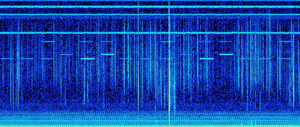
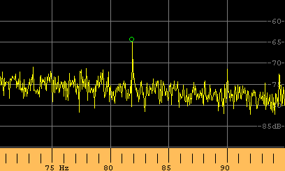
In the following four images the mechanism
is clear, where a 100 minutes recording have been analyzed in spectrum
view and in waterfall (spectrogram) view with different resolution and
then with various number of FFT points. Where it seems to be only noise
it appears a clear 82 Hz signal: we are analyzing the same file! Different
frequency resolution gives different signal/noise ratios. This effect is
called "FFT gain" in literature.
 |
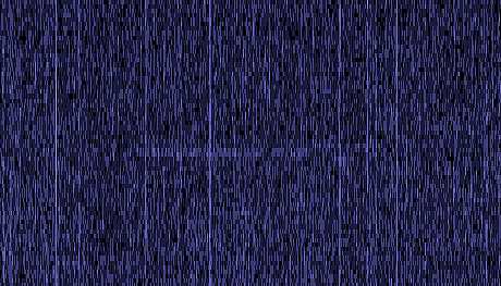 |
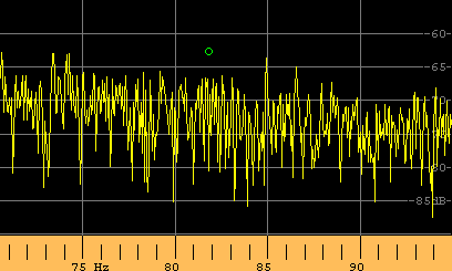
| Spectrum obtained with 2048 FFT points, 125mHz resolution. The green little ball point out where the 82 Hz signal may appears. | Spectrogram
obtained with 1024 FFT points, 250mHz resolution
Frequency range 78 Hz - 86 Hz. Appears a very weak trace. |
 |
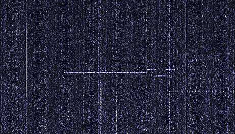 |
| Spectrum obtained with 16384 FFT points, 15mHz resolution. Despite of the same file analyzed, now the signal is clear. | Spectrogram
obtained with 4096 FFT points, 62mHz resolution
Frequency range 78 Hz - 86 Hz. Best view with the spectrogram. |
SETTINGS MISTAKES
As we saw, a FFT signal is determinate by mathematics rules which are very precise. Many programs do some controls on incoming data (as "Spectrogram" and "Spectran"). While some other ones accept every kind of given parameter (as SpectrumLab): we need to know what we are doing before type enter. Faults of use are due of incorrect association between calculated data of FFT and their video representation in pixel.
Apart parameters time/frequency described before, correctly chosen (even if is not a true mistake) exist some settings which are incorrect.
a) MISTAKES IN A REPRESENTED
FREQUENCY BAND
A 512 points FFT gives origin to a graphic representation
of 256 points if the side image is of 256 pixel. If the side image
is in side frequency 256 pixel, we've the association 1 BIN
1 pixel. If we reproduce the full screen spectrogram
(1024-766) by reproducing 256 bin on 768 pixel we'll have the association
1 BIN 3 pixel. Pixels will be equal by groups of 3.
If we do an FFT of 65000 points the represented BIN will be 32.000. In order to visualize the whole analyzed band ( by following the association 1 bin 1 pixel ) we need a 32.000 pixel screen dimension.
It is correct to represent on the screen a number
of bin accorded to the available pixel . With a
many points FFT the represented band must be reduced. A good
rule could be :
|
Frequency span = Frequency resolution x available pixels |
Two practical examples about a 256 pixel high image:
FFT
512 pts, SR=44100, Freq. Resolution=86.1 Hz, Band =86,1x256= 22050 Hz
FFT 65536
pts, SR=44100, Freq. Resolution=0.67 Hz, Band =0,67x256= 172,2 Hz
B) MISTAKES SETTING SCROLL
TIME
The Time Scroll setting say every how often on
the image must appear a spectrogram line.
It's better if Time Scroll is as long as the Buffer
filling time. A shorter Scroll time time makes an overlap, that is a short
signal is faded and so is represented on several lines. So the represented
time is longer than the real one.
Usually an overlap up to 4 gives an acceptable
representation of the analyzed signal.
|
Time Scroll = 1 / Freq. Resolution = FFT point / Sample Rate |
At example:
Sample rate 44100 S/sec and FFT of 1024 PTS.
The real time scroll will be: 1024/44100 = 0.0232
sec, or better 23.2 mS.
It means that the program will calculate an FFT
strip every 23 mS: if we set a scroll time of 2.3mS we will obtain 10 vertical
lines of the spectrogram with almost the same representation.
But we can give the following representations:
 |
1° representation
(correct)
Setting 23mS as time scroll we will have 1 FFT representation every 1 pixel strip |
|
 |
2° representation
(inadeguate)
Setting 100mS as time scroll we will have 4,3 FFT strip every 1 pixel strip, losing many informations |
|
 |
3° representation
(inadeguate)
Setting 2mS as time scroll we will have 11,5 pixel strips every 1 FFT strip (obtaining an overlap effect) using many pixels to reproduce same data. |
An exaggerated overlap, for instance 25, gives the idea that the analysis gives more details on the analyzed signal: is because the spectrogram runs quickly; the same data are reiterated more and more times on the FFT line, wasting space on the image which the signal represents. For some applications (like in the radio amateur community), a carefully selected amount of overlap in the FFT input data is beneficial to decode slow morse signals on the waterfall screen. There are specialized programs which do this selection automatically, others (where "everything" is adjustable) require more care to select the right parameters.
If we want to compare in optic way, let's take a
picture done with a 60° view. If we take the image and
stretch it in horizontal way three times, we'll simply obtain a distortion
image and not a 180° viewing.
FFT PROGRAMS
They are many, but we'll end to name the main three freeware ones.
SPECTROGRAM
(version up to 5,7), of Richard Horne
The first one, talking about time, and for sure
the most used. Limited in its functions ma complete at the same time.
It gives itself to FFT the pixels, without mistakes (Time scroll
free only). Easy to use, the best for beginners.
Download from: http://www.visualizationsoftware.com/gram/gramdl.html
SPECTRAN
of Alberto Di Bene and Vittorio De Tomasi
Different graphic, it look a bit like a measuring
device, it gives higher resolutions. Best if with a RF receiver even
for radioamatour applications. Easy to use it gives correct visualizations
(don't accept unsuitable data)
Download from: http://www.weaksignals.com
SPECTRUMLAB
of Wolfgang Büscher
At the present the most complete for signal analysis.
Give every kind of real time and post process elaboration but can also
accept incorrect data input. Some active filters allow VLF reception
also when hum noise is very high. The best for unattended operations. Not
for beginners: we need to know something about FFT parameters before use
it.
Download from http://www.qsl.net/dl4yhf
CONCLUSIONS
Let's stop here: about FFT many books have
been written, full of formulas. In this article we've written few
of them: the main ones.
We've tried to explain FFT analysis basic concepts:
this will be useful when the programs will be practically used.
Many Thanks
to:
Andrea Bertocchi, for English translate
Wolfgang Schippke, for technical revise