| Design
of High-Performance Magnetic Field Sensors
for ELF – LF Signal Reception and
Characterization by Evan Iverson, Tucson, Arizona (written December 1994) Executive Summary We present an approach to the design of state-of-the-art, magnetic-field sensor systems that can be optimized to detect extremely weak electromagnetic signals over a wide frequency range from ELF through LF (3 Hz – 300 KHz). Our design approach provides a balance between performance and fieldability and offers several ways to trade off design features to achieve optimal solutions for different applications. Features of our approach include an SNR-optimized antenna and front-end amplifier to provide femto-Tesla (fT) sensitivity; a flat, wide-bandwidth frequency response; and high dynamic range. This minimizes requirements for high back-end DSP processing gain (i.e., long integration times). As an example of the achievable performance, one point design tailored for ultra-sensitive, wide-bandwidth characterization of either natural or man-made signals in the ULF – LF bands provides the following capabilities:
Introduction Radiometric and polarimetric measurements in the electromagnetic spectrum from a few Hz to a few hundred KHz can yield significant insights into ionospheric and magnetospheric dynamics. This realm of radio science exhibits a rich range of natural phenomena, such as Schumann resonances; whistlers and other “spherics” resulting from lightning discharges [1]; polar chorus and auroral hiss; and propagation enhancement due to sudden ionospheric disturbances (SIDs). Man-made signals in this portion of the electromagnetic spectrum include navigation signals such as Omega, LORAN and nondirectional beacons (NDBs); communication signals intended for reception by submarines; and standard time and frequency signals. Providing high-sensitivity receivers for signals in the ELF, SLF, ULF, VLF and LF frequency bands (3 Hz to 300 KHz) presents significant challenges. Some approaches are based on electrically small E-field or B-field antennas, often resonated to the frequency of interest, and typically employ high-impedance amplifiers to minimize voltage-signal loading. Performance tradeoffs are usually not well understood and total system noise performance is almost never optimized for the specific signal(s) of interest. Surprisingly, no published technical paper has been found that provides a sensitivity-based analysis and design of electrically small antennas for weak-signal applications. The goal of this paper is to provide an approach for the design of magnetic-field receiver systems for which high sensitivity, wide bandwidth, and high dynamic range are essential. The natural noise floor in the ELF through LF range is reasonably well characterized [2]. The noise measurements indicate an average spectral density of ~1 For purposes of illustration, consider a situation for which the local natural noise density is ~5 The signal-detection challenge, however, is also affected by man-made interference and natural impulsive noise. This drives the need for high dynamic range in addition to high sensitivity to provide the maximum SNIR possible for the analog signal so the requirements on back-end DSP processing gain are reasonable. Finally, some applications may also require a large relative bandwidth to capture signals with relatively fast risetimes, to enable signal search using DSP techniques, or to support the characterization of phenomena that span a relatively large frequency range. Designing an antenna/receiver system that meets these challenging sensitivity, bandwidth and dynamic-range requirements while keeping the hardware relatively small and easily fieldable is a significant challenge. The technical approach we present below enables these challenges to be address in a rigorous manner.
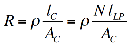
Antenna Technical Approach B-field sensing can provide advantages over E-field sensing for high-performance receivers in the ELF-LF range. One advantage is the ability to shield B-field antennas from sources of local E-field noise, such as electrostatic discharges due to wind and rain or switching power supplies. Other advantages may include ease of construction, ease of calibration, and antenna null depth. However, in applications that require operation in noisy industrial environments in which magnetic induction is significant, E-field sensing may have the advantage. This paper does not include an analysis of the B-field vs. E-field performance tradespace because it is highly dependent on the application and receiver environment, but focuses only on the optimal design of B-field antennas and amplifiers. B-field antennas are conductive loops, and when they are electrically small they provide an electromotive force in response to a time-varying magnetic flux through the surface delineated by the loop according to Faraday’s law of induction. Consider a loop antenna comprised of N identical turns of a thin conductor (wire) in a uniform magnetic field B. The open-circuit, terminal-voltage magnitude V in response to a harmonic B field with frequency f can be shown to be where A is the loop area, and An electrically small loop antenna exhibits both a resistance R and an inductance L that depend primarily on the parameters of the loop. The ohmic resistance, neglecting skin effects and proximity effects, which can be shown to be minimal at our frequencies of interest, is given by where Now, consider the magnitude of the short-circuit current for an electrically small loop antenna. With best alignment of the dipole antenna response pattern ( This is a classic single-pole, high-pass-filter response with a 3-dB corner frequency at where The issue of noise and sensitivity will be covered next, but first an additional important observation is stated. Given a fixed loop shape with area A and a fixed conductor mass Receiver sensitivity, which determines the minimum detectable signal (MDS), is limited by antenna thermal noise and amplifier voltage and current noise. The sensitivity of the antenna alone can be defined as the B-field equivalent of the thermal voltage noise density, This indicates the antenna becomes more sensitive ( Substituting Equation 2 into Equation 5 with the conductor length expressed as Here The additional expressions for
Amplifier Technical Approach The antenna-sensitivity relationships presented above were derived by considering the B-field equivalent of the thermal noise density. The primary goal, however, is to optimize the overall system noise figure to provide an SNIR that is not limited by the antenna/amplifier combination while providing features such as wide bandwidth, high dynamic range, and fieldability that are important for the application. As mentioned earlier, the antenna/amplifier design could utilize the unloaded, open-circuit antenna voltage. This requires an amplifier with an input impedance much greater than the antenna source impedance Returning to the design concept associated with Equation 3, we focus on amplifiers for which the input impedance can be reduced to a very low value. One approach is to use an interstage transformer along with a balanced, common-base amplifier topology for the first stage. That approach, however, adds considerable complexity to the design and introduces additional rollofs and resistance. This increases the corner frequency Revisiting the ELF-LF sensitivity optimization problem with consideration of current technology indicates that the design tradespace can now be extended to include the use of ultralow-noise operational amplifiers in a transimpedance configuration. This has led to the development by the author of an antenna/amplifier performance model for ionospheric and magnetospheric research in the ELF through LF spectrum. When considering device options for an ultralow-noise, transimpedance amplifier, operational amplifiers from Analog Devices, Burr Brown and other companies meet requirements. New device designs are being optimized for operation at low equivalent source impedances. They are anticipated to have an input-referred voltage noise density of ~1 Our antenna/amplifier technical approach optimizes the antenna, using the equations presented above, in relationship to the transimpedance amplifier V/I gain and input-referred voltage and current noise densities. This results in sensitivities at the
Antenna/Amplifier System Design Example As a design example, we consider performance requirements to provide an ultra-sensitive capability to support broad-bandwidth characterization of ULF/VLF phenomena such as whistlers. The key requirement is a We then balance the antenna noise voltage density against the input-referred voltage and current noise densities for an ultra-low-noise operational amplifier that is optimized for operation at low equivalent source impedances. This involves a number of tradeoffs including transimpedance amplifier V/I gain, system transducer gain, closed-loop bandwidth, and dynamic range. Choosing the number of loop turns used to distribute the required copper mass,
Summary and Conclusions We presented an approach to the design of state-of-the-art, magnetic-field sensor systems that can be optimized to detect extremely weak electromagnetic signals over a wide frequency range from ELF through LF (3 Hz – 300 KHz). Our design approach provides a balance between performance and fieldability and offers several ways to trade off design features to achieve optimal solutions for different applications. Features of our approach include an SNR-optimized antenna and front-end amplifier to provide femto-Tesla (fT) sensitivity; a flat, wide-bandwidth frequency response; and high dynamic range. This minimizes requirements for high back-end DSP processing gain (i.e., long integration times).
References [1] Robert. A. Helliwell, Whistlers and Related Phenomena, Stanford University Press, 1965. [2] E. L. Maxwell and D. L. Stone, “Natural Noise Fields at 1 cps to 100 kc”, IEEE Transactions on Antennas and Propagation, AP-11, No. 3, pp. 339-343, 1963. Return to vlf.it index
|
 [2]
[2]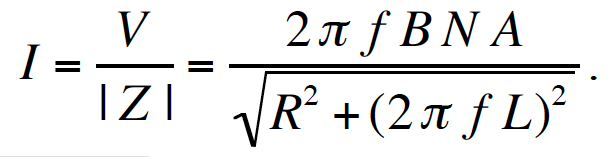 . [3]
. [3]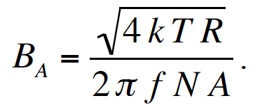 . [5]
. [5]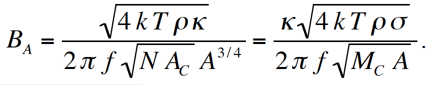 . [6]
. [6]