|
Signals
in the ELF-Range
Part III-1 Kurt Diedrich, Franz-Peter Zantis (Please read part one and two for introduction) Contents:
Recalling
In
the first two articles, we described a number of
strange ELF-Signals we
received in a small village located in the Eifel
mountain region in Germany.
We found out, that these obviously manmade signals
based on magnetic waves
must have their origine a few feet under the
surface of the street located in front of the home
of one of the authors,
Kurt. Meanwhile, our investigations went on: we made
a number of new discoverings
and perfected our receiving methods – but
still we did not yet
find out where all these signals come from.
Our
first idea, the signals could be created by currents
passing through water
and gas pipelines or telephone wires was wrong:
Measurements made along
these sources within the house and also outside
in the village brought no positive results: The
signal source seemed to
have nearly a dot shaped area and obviously was
located below a small intersection
within the village (see also chapter Bearings).
Based
on this and also on the fact, that the same signals
can also be received
by metal sticks put into the ground, we developed
the theory, that wide
spread signal currents all over the region could be
received by water pipes
like radio antennas are doing this in the open air.
If, at certain locations,
these pipes are grounded by being wired to a lower
potential, the currents
of all antenna -pipes are accumulated and conducted
by one cable to ground.
The currents through this wire then could be so
strong that they are radiating
the magnetic ELF-signals we receive. Butt this is
still a theory which
yet has to be proofed and doesn t explain the
origine and the purpose of
the signals.
In
early 2006, because of personal reasons, Kurt had to
move away from the
little village in the Eifel mountain region, where
all those interesting
signals partly described in the first two articles
could be received. His
new domicle (at Alsdorf-Mariadorf) is located about
30 kilometers north-west
from his old living place and only 800 meters away
from the place where Franz
Peter lives. So it was possible for the first time
to carry out systematic
measurements at the sime time from two points not
far from each other.
But
let us tell the story from the beginning: What did
we expect? At first, Kurt
did not know at all if he could receive any signals
at his new living place.
After a few days of testing, the situation was a
little bit clearer: There
were signals, but they had been less strong as those
at the old living
place and they were less spectacular. The main
signal which could be received
was the well known Heartbeat-Signal. Apart from
this, new signals described
later appeared and disapeared again within a few
weeks, but most of them
(there were a few exeptions) were only a few dB
above the noise level.
These facts gave us the idea, that here, like at the old place, there must be a comparable signal source, which here only had a bigger distance then the one in Hürtgenwald. At first, we were rather sure that it even would be the same source that Franz Peter can receive at his home (800 meters away). Though we had no proof, we intuitively did not believe that within such a small distance, more then one signal source could exist. But first measurements at the same time were disabusing us: Even at a such relatively small distance of 800 meters, completely different signals could be received at both stations: There were specific signals which were typical for each of the two locations, and there were signals like the heartbeat signal, which could be received at both stations, but at completely different times. In addition, at both stations we also could receive the goose signal we discovered at Hürtgenwald, but less strong. This was the only signal we could receive synchronously. The most spectacular new signals at the new living place of Kurt are signals which sound like a robot voice, (still) appearing three or four times at the evening, then a sound comparable to the foghorn of a big ship and also a number of sounds like birds voices. A very strong signal appeared during the first six month of the year 2009, in its structure looking similar to the goose signal, but extremely strong and only appearing each day from fall 2008 until summer of 2009 at five minutes past two o clock PM. Having discovered that there are completely different signals within such small distances of 800 meters, we tried to find out if different signals could also be found within even smaller areas. They can: A measurement at a parking lot only 100 meters away from the home of Franz Peter showed a sequence of heartbeat signals which differed completely in their structure and time pattern and which could be registrated at different hours of the day. Encouraged by these results, we started to carry out measurements at nearly every place in the village and in the neighbour villages, where we could make a stop with our cars. The measurement system (receiver, antenna, PC) was installed inside the car. So we used public parking lots in front of supermarkets or parking areas at the border of forests for people who like walking. We also made measurements in a number of different towns and villages all over Germany. In each town, we could find typical signals which could not be recieved in other towns. We also found the typical heartbeat signals, which probably my be present over the whole country and at least in southern France, where one measurement was made during a holiday trip. That all these measurements in different towns would not match among each other was a fact we could understand and explain by the big distances of hundreds of kilometers. But the fact that all those dense measurements made in one region didn t match at all still seems very strange to us. In addition, the fact that we could not receive any of the signals in question beyond populated places (in fields and forests) could be explained by the theory, that gas and water pipes work like big underground antennas. If this theory is wrong, the ELF-signals must be created within populated places by some machines. But what kind of machines? It doesn t seem evident that each village or even street in this village uses its own machine to create a typical ELF-Signal. What kind of machine could that be? Machines used by civil people like refrigerators, TVs, radios, cellular phones and PCs don t create signals in the ELF-range. And what about machines with motors like dust cleaners, laundry dryers or washing machines? The all are functioning by the same principle. So if they produce ELF-waves, the corresponding signals should be equal at each measurement location. But this is not the fact. And why do some signals only appear for a few days, weeks or months and then disappear again? And why can some be only received for a few minutes at the same hour each day?
Localisation
of the new signal sources
Until
now, it was not yet possible to find out precisely,
where the sources of
the signals registrated at Mariadorf are located. At
Hürtgenwald it
was easier because of the fact that the source
accidently was located immediately
in front of the house where Kurt lived. If the
source is located in a bigger
distance, bearing of ELF-waves in question
becomes difficult because the lines of the magnetic
flux all run vertically
and there is no correlation between geographic
direction and line direction
(see also chapter Bearings).
So,
only wide spread,
dense measurements covering the whole region (mapping)
will bring further
information.
Summary
In
populated aeras,
there probably must be sources spread over distances
of approximately 50
meters, which emit mangetic waves in the ELF range
with a relatively high
intensity. These waves can be interpreted as different
signals with partly
complex time and frequency patterns which can be
classified into different
groups.
Most
of the sources
are characterized by their own typical signal
patterns. Some of these patters
also appear at other sources, but never at the same
time.
Only
one single pattern
(see goose signal , Part I and II) was received from
2002 until 2007 at
all locations in the Aachen region synchroneously. The
point of its strongest
intensity was located in Hürtgenwald (Eifel region).
Even in a distance
of 40 km, at Heinsberg, it still could be registrated.
Very strange: Since
the middle of 2007, the signal suddenly vanished.
Then, in fall 2008, it
could be received again for a few weeks. Since that
time, it seems that
it disappeared completely.
Meanwhile,
at many different places in Germany, measurements
have been carried out.
In theses cases, each location (but only in housing
areas) also had its
typical signals, except the heartbeat signal, which
could be received at
all places (and also in southern france) at
different times and with different
structures.
Model
of explanation
Metal
sticks of approximately
40 cm length sticked into the ground are able to pick
up electrical potential
differences of earth currents. By using such
additional electrodes at our
measurement locations, we could show that the signals
that we recorded
with our receiver for magnetical waves and the current
signals measured
by the electrodes were identical. Facing this fact, we
assume that the
signals in question propagate through the surface of
the earth by very
low large scale currents, which are not strong enough
to create magnetic
fields.
Long
metal pipes,
e.g. for water supply, then could work like long wire
antennas of old fashioned
radios. At some location, these long water pipelines
may be grounded. That
means that they are connected via thick cables to a
point of lower potential.
At such places, the earth currents catched by the
pipes could be accumulated
to a current of a higher density, which is able to
create a magnetic field
of sufficient density. This would
explain why
signals only appear only at single locations within
housing areas.
Our
latest measurements seem to indicate that the source
of the signals can
be found in these grey metal cases standing at the
sidewalks
in nearly each little lane or street of each town or
village. These cases
contain, at least in Germany, the distribution nodes
of the mains-, telephone-
and internet supply for the surrounding. At
star-shaped networks it may
be possible that the signal currents are collected
by the radial wires
and concentrated in the center point.
To
proof this theory
(which is not yet be done until now), it is important
to carry out electrode
measurements out of housing areas in fields or
forests. By using electrodes,
there also should be detected signals comparable to
those in villages.
Exclusions Home appliances, privately used machines, mains control signals and railway control signals can be excluded as signal sources:
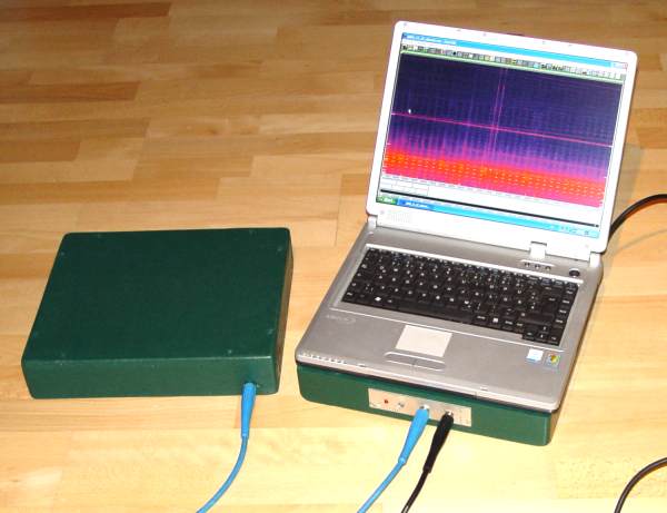
Receiver
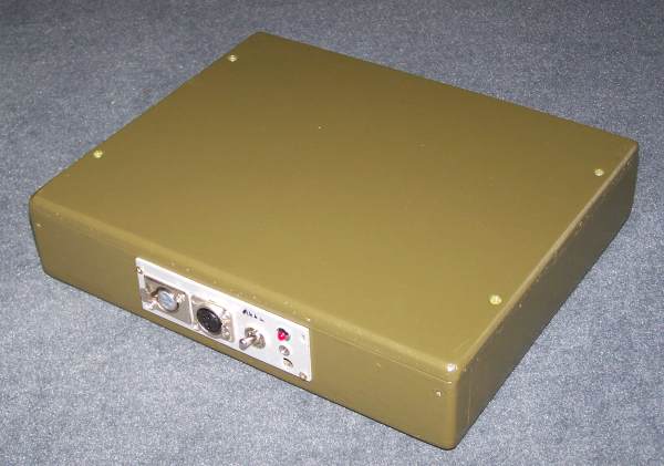
Figure
above: Mobile use
by
rugged case
Figure above: One of the first prototypes with receiver, small coil and notebook The receiver consists of a ring shaped coil antenna, followed by a high gain voltage amplifier and a high performance low pass filter of 42 dB per Octave to cut out the disturbing 50 Hz hum. The output signal can be fed into any default PC sound card and is recorded, displayed and converted into a wave file by a special softare written by the authors.
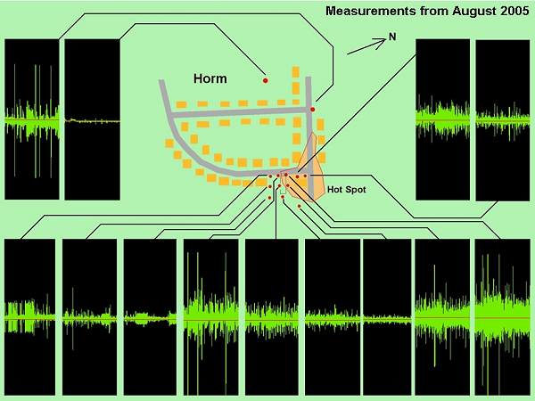
Bearings When I discovered the first signals in question, I already asked myself where they could come from: Directly from underneath the house, from the garden or from far away? To find an answer, I carried out different measurements at different locations in the house, around the house and in the neigbourhood up to a distance of approximately 200 meters on a childrens playground at the border of an agricultural field. In my home and in the garden of my home the signals were very strong. The bigger the distance from my home, the weaker the signals got. On the playground mentioned above, there nearly were no signals to receive. The computer drawing based on these results shows a schematic map of the small village and the time signals I received at the different measurement locations. The amplitudes shown in the time signals indicate the intensity of the signals at the different spots. Regrettably, it is not possible to compare the results precisely: The signals are all different because they were not made at the same time.
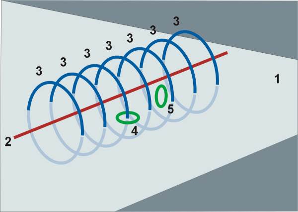
Figure: Different measurements made in the environment of the base The result of these comparisons showed me, that the signals must be local and could not come for example from far away military submarine transmitters somewhere in the USA or Russia. One problem still remains: To create a map of signal intensity with a high resolution, it would be necessary to carry out measurements within a large scale grid with very narrow matrix dots of approximately 10 to 20 meters. As one single measurement takes at least half an hour, it is easy to imagine that all our holidays and spare time would not be enough to do this. In addition, the biggest part of the environment there was private. Indeed there exists a solution which is much more easier: Bearing! When using this method with radio frequencies, you turn a special antenna until the intensity of the received signal goes to zero or to a minimum value. If this is the case, the bearing antenna points to the direction the signal comes from. Bearing with maximum values would also be possible, but a little and absolutely nothing are better to distinguish than maximum and a little less than maximum . If you carry out two bearings at different places and copy the appropriate directions to a map, the source of the signal is located at the crossing of both lines. This method is very easy with radio waves of high frequencies, but it is difficult within the ELF-Range because the direction of the streamlines of the magnetic field have to be considered. The picture below shows a horizontal wire (2) with an electric current at the surface of the ground (1). The current creates a magnetic field, where the streamlines (3) can be imagined as vertical rings. The two small rings (4 and 5) are our ring shaped coil antennas. In position 4 (the coil is in a horizontal position), the reception is always maximum, because the streamlines of the magnetic field are at right angle to the surface of the flat coil. As the coil is rotation symmetric, there is no use in turning it around its vertical symmetry axis: The intensity of the received signal would not change. So in this case you can not find out from which point of the compass the signal is coming from. Different results in reception you will get by changing the coils position between 4 and (vertical position) 5. If the coil is in a vertical position, the streamlines of the field nearly do not cross the circular area of the coil. So, by moving the coil between these two positions, you only can find out the vertical direction of an appropriate signal (under the preconditions of the picture below). This may not be very helpful at the first glimpse, but if you have the ability to measure from different altitudes (a high building or a tower) in the neighbourhood of the signal source, reliable bearing results may be possible too. If you got the vertical angle, you can start to optimize your result by carry out measurements now in the compass directions with keeping the vertical angle you found before. Keep in mind that this will only be possible, if your position is different from the plane (1) in which the emitting source (2) is located, or with other words: if the vertical angle is different from zero (horizontal).
Figure: 1: ground, 2: wire, 3: streamlines, 4: horizontal coil, 5: vertical coil Experiences have shown that you still get good measurement results if you take angle steps of 10 degrees around the horizontal and vertikal axis to approach the right direction. Otherwise, the measurements (each of them about half an hour) would take to long. If you have got any result, you can start to carry out your measurements more precisely.
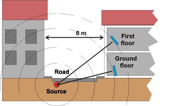
Figure:
Finding the source by two bearing measurements from
the first and the second
floor of a house.
As
I was lucky to have the signal source (accidently)
just in front of the
house I lived, I was able to determine the source
very precisely by measurements
from the ground floor and the first floor (picture
above). As this was
a very rare case, usually it will not be so simple
using bearings to find
the source of the ELF signals. I even could find out
that the source must
be about half a meter below the surface of the road
near the border of
the sidewalk. Unfortunately I could not determine
the length of the source
and so answer the question if the signals came from
a spot or a kind of
pipeline.
At
first we were
disappointed, because we believed that we had found a
simple, natural explanation
for the signals: Data transfer along water and gas
pipelines, transmitted
by the water or gas supply companies to control their
systems. To find
out if that s true, we carried out measurements all
along the streets in
the small village where we expected water, gas and
other supply systems
to be located in the ground. The result was very
strange and caused a number
of new questions: At all other measurement locations
along the course of
the pipelines, no ELF source could be detected: All
the signals (and also
the background noise) we received came from a single
spot in front of the
house I lived. If the signals would be propagated by
the water, gas or
telephone lines, they must be receivable all along
these lines, which is
not the case. The picture below shows a simplified map
with all measurement
points along different streets of the village. The
place, where the signals
could be received, is marked (ELF Spot).
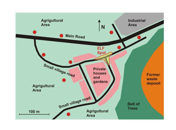 Figure:
Map of the village where the measurements have been
carried out. The dots
show the different locations where we could not
receive any signals along
gas and water pipelines. Only in the area ELF Spot
the signals were present.
Facing the measurement results, we may estimate that the center of emitting is only accidently in a location which is also crossed by supply pipelines and that there is no relation between the pipelines and the signals or that, by certain unknown circumstances, only small parts of the municipal pipe or wire systems are emitting signals Later
measurements
showed, that the emission of ELF signals has something
to do with municipal
supply systems: As already mentioned, the signals can
only be detected
in urban housing areas. Regrettably, by lack of time
we could not yet proof
this theory until now.
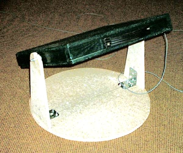 Figure:Simple bearing antenna with inclinable coil (in the case)
Signal Analysis As already mentioned, a special software, written by the authors, is demodulating the carrier and writing the signals as wav-files on the notebooks hard disk. The recorded files can be analyzed by an analyzing software with an FFT vs time analysis. Due to our method of data processing, the signals are transferred in a range that is 160 times higher than the original ELF frequencies and become audible. This means that a signal which was recorded over 160 minutes is played back in one minute. All important frequency components of the ELF signals are arranged over the complete audio range and not only to be seen on screen but also to be heard.
Scaling
The
frequencies in all FFT vs time diagrams are lineary
scaled. The scales
of the levels (intensity) are logarithmic.
The frequency range (Y-axis) goes from 0 to 100 Hz
in the original files.
The range of interest is limited from 0 to 25 Hz. In
some of the screenshots,
the 50 Hz mains line can be seen clearly and be used
as a reference. As
the levels at the 50 Hz range in the diagrams are
attenuated about 36 dB
in comparison to the 25 Hz range (because of the
filter), you can easily
see, how low the levels of the registraded signals
are in comparison to
the magnetic fields created by the 50 Hz mains.
Without
the attenuation
by the filter, the 50 Hz mains signals would
overmodulate the receiver.
In most of the diagrams shown in this documentation,
the Y axis is limited
to 25 Hz as there were no intersting signals found
above this frequency.
One
strong line in
the lower range of the diagram is the 16 2/3 Hz line
of the german railway
supply voltage, which can be measured up to 6
kilometers away from the
nearest railway line and which can be used as a good
reference line. Also
this line, if it exists, can be used to check the
function of the receiver,
if no other signals are present at a certain location.
If ne next railway
line is nearer then 1 kilometer, measurements will be
overmudulatet by
the railway frequency. Filtering in this case would
not be very useful
as the railway frequency appears in the same range as
the frequencies of
interest.
As
the Screenshots
of the Analysis do not contain any frequency scaling,
the frequencies of
interest are printed in the diagramm if necessary. In
many screenshots
you'll find a scaling of the X axis, given in samples.
If the sample rate
was 200 Hz (which was the case at all measurements),
the time difference
between two values on the X axis can be calculated as
follows:
sample-value
/ 200 = time in seconds
New signals and new discoverings in old signals In this part (III-1) the focus is set on the heartbeat signal. This signal appears regulary and could be recieved neary at each measurement location within germany. In part III-2, an number of additional signals will be described precisely.
Heartbeat signal This signal was already described in our previous contributions: It seems a little boring as it never seem to change in its structure. Its spectrum shows, that it has a rectangular waveform and a frequency which is a little higher than 1 Hz. This signal is transmitted for some minutes (realtime), followed by a pause which is approximately as long as the signal itself. Then, the same procedure starts from the beginning. What's irregulary is the time the signal is present: The lenghts of the signal-pause sections differ continuously and were never equal in years of measurement. Also, the numer of transmissions and the time of their beginning over a day is always different and it seems, that there is no system behind it. The signal appeared for the first time in the year 2004 at that time only in the morning hours between 6 and 7 AM, but then it also started and ended each day at different times. In the course of the following months, it appeared more often and can meanwhile be regarded as a kind of noise, covering other interesting signals. In addition, this signal meanwhile could be received everywhere we carried out measurements within a wide range of Germany and, as already mentioned, at one location in southern france. Even in one village, the home village of Kurt and Franz Peter, heartbeat signals could be received independently (at different times with differnet lengts) in a short distance of lass than 100 meters. In most of the cases, the spectra of the signals were identically. In a few cases and not long ago, for the first time we regsitrated signals with a frequency a little lower than usual at the location of Franz Peter.
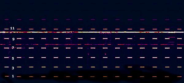
Figure:Heartbeat signal spektrum. One beep lasts about 1.5 minutes in realtime. The figures indicate the range of the harmonics, which are typical for the rectangle or square wave function. Because of physical limitations of the coil antenna, frequencies below approximately 5 Hz are attenuated. This effect is widely compensated by an extra linerisation filter, but it could not be supressed completely, which can be seen in the lowest lines in the figure above. In the upper range of the figure, the 16 2/3 railway line can be seen very clearly. Above this line, the low pass filter of the receiver starts with its attenuating.
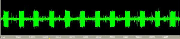
Heartbeat
time signal
Important
notes to the heartbeat signal
(Only)
in combination with the heartbeat signal, short and
irregular sine signals
of 16 2/3 Hz and with a higher level as the
heartbeat signals can be received
at all our measurement locations. As these signals
were also received at
locations, where no railway signal was present and
no railway lines were
in the neighbourhood, these 16 2/3 Hz Signals seem
to have no relation
to the railway supply system.
The
following figure shows an example: At first take
a look at the time signal in the middle: Besides the
known heartbeat signals
you can recognize four bars with a higher amplitude.
The time signal above
shows the time expanded structure of one of these
bars : A clear sinewave
of 16 2/3 Hz.
The
spectrum of the
whole time signal (third figure) proofs that its
really a sinewave with
a higher intensity (the lines are much brighter than
the ones of the heratbeat
signal). Sometimes, the signal of 16 2/3 Hz is
modulated in its amplitude
by a sinewave of a lower frequency.
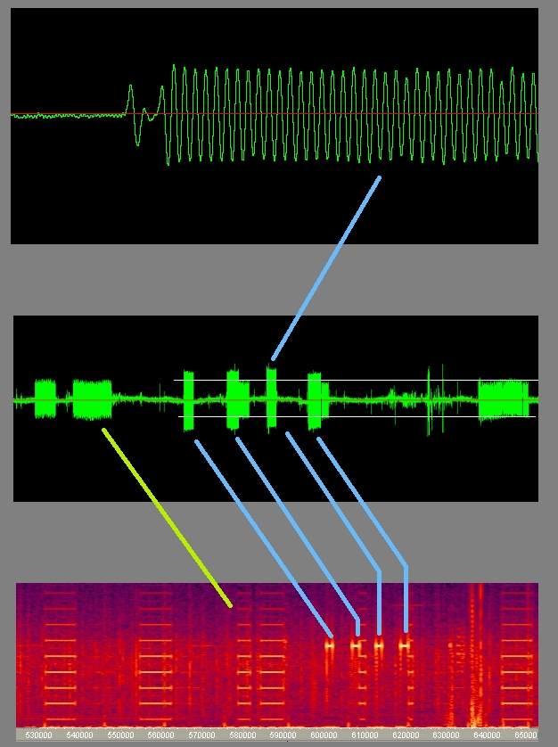
Strong
16 2/3 Hz signals in combination with
heartbeat
signals
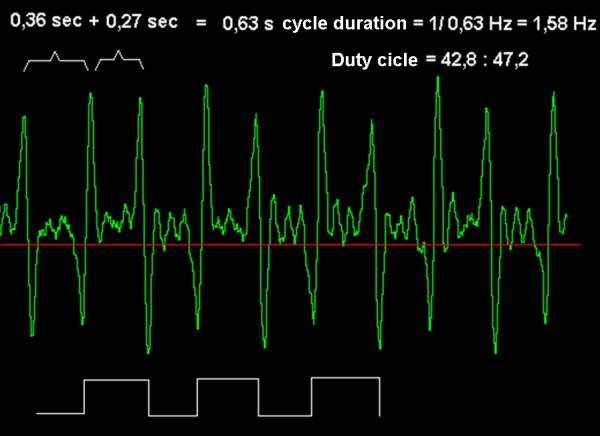
Examination of the signal parameters The picture below shows a zoomed section of the heartbeat time signal, which consists of pulses changing from negative to positive alternately. Such pulses are created for example if a rectangular signal is differentiated. At first we thought that this differentiation was done by the coil antenna, but when we were working with the electrodes, we got the same waveform for the ground currents. By the way for the spectrum analysis there is no difference between a signal and its integrated copy: A square wave signal and a differentiated square wave signal have the same spectrum. Measurements have shown that the heartbeat signal (with few exceptions) always had a frequency of 1.58 Hz. The duty cycle was asymmetric between 43 and 47 percent.
Figure: Duty cycle of the heartbeat signal Note:
For English spreaking readers, the comma in some
figures must be replaced
by a dot .
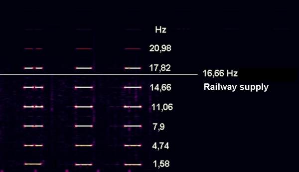
Figure:Zoomed
part of the heartbeat signal spectrum with the
frequencies of the harmonics.
Uneven harmonics are typical for square waves.
We
do not know if
the original emitted heartbeat signal is pulse or
rectangular shaped, but
we suppose it could be a rectangular signal, created
by switching on and
off a DC current alternatively by some kind of
electronic circuit or machine.
Any
information in the heartbeat signal?
A
first look at the heartbeat time signal lets you
suppose that it is completely
of technical nature and does not contain any
information: The structure
is equal at each time section. In addition, we could
not find any trace
of phase modulation: The duty cycle is always
constant within one transmission.
By
comparing the number of pulses in different bars
(beep sections), we discovered,
that they differed between a number of 114
and 122. This may be accidently, but if this is any
information, it would
not be very efficient. As one beep lasts one and a
half minute in real
time, the data transfer rate would be very low.
In
the figure below, the beep phases were cut into
pieces of 10 pulses to
get a better impression of the different number of
pulses in different
beeps.
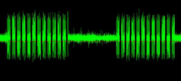
Figure:
Counting the pulses by cutting the signal into
pieces of ten pulses
Mapping
of
heartbeat
signals
As
the signal is dominating in the region of
Aachen, we asked if this signal was also present in
the rest of the country.
As we had not enough time and money to carry out
systematic explorations,
we used holiday and business trips for large scale
measurements. In the
following, there is a list of all the locations we
could carry out measurements
apart from Aachen sometimes in hotel rooms and
sometimes at outdoor locations.
The intensiy of the signals doesent give any
information of the intensity
of the appropriate emitting sources, because we did
not know anything about
the distance to it.
Location:
Year
Result
Dudweiler
(Saarland):
2005
very clear
Dremmen
(Rheinland):
2005
very clear
Heimertzheim
(near Bonn):
2005 extremely strong
Bübingen
(Saarland):
2006
clear
Büsum
(Schleswig Holstein): 2006
very low
Allershausen
(Bavaria):
2006 very clear
Gerlingen
(near Stuttgart): 2007 low
St.
Marie (southern France): 2007
very low
Bierbergen
(near Hildesheim): 2007 low
Gressenich
(near Aachen):
2008 clear
Eschweiler
(near Aachen):
2008 clear
In
the year 2009, the list was continued with additional
locations and comparable results.
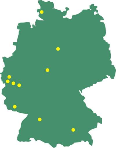 Figure: The dots mark the regions where we had the ability to carry out measurements. Everywhere the heartbeat signal was found As
well as at Büsum (northern Germany) as at St. Marie
(France), the 16 2/3 Hz signal of the railway supply
was completely missing.
Nevertheless, the strong 16 2/3 Hz signal in
combination with the heartbeat
signal, which was described above, could be detected
clearly.
Comparison
of intensities
The
following figures show the spectral
values of
the heartbeat signals from the list above and in
the same range. As already
mentioned, the intensity does not say anything
about the energy of the
emitting source as their distances to the receiver
were unknown in all
cases. Nevertheless it is interesting, that the
time and frequency structures
of the different signals are all the same.
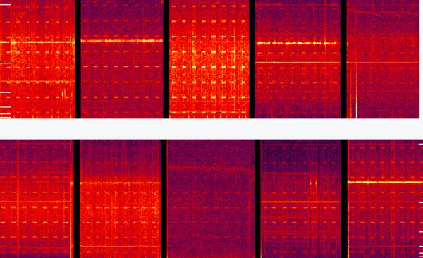
Figure:
Relative comparison of heartbeat signals received at
different places in
Germany. The intensity in the diagrams says nothing
about the actual intensity
because the distance to the signal sources was
not known.
Please read Part III-2 to learn more about other ELF signals received by the authors. Kurt Diedrich / Franz P. Zantis
September 24, 2006
Return to the main index of www.vlf.it |