Strange features of the whistler signals
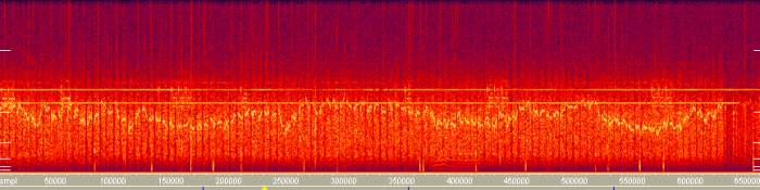
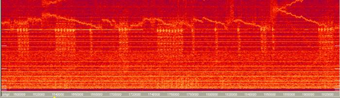
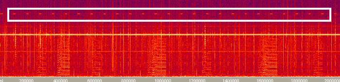
The figure below shows the time structure of the signals over a longer period of time. The transmission begins with a longer sequence of signals, consisting of about 60 whistles. Then, after a break which corresponds to approximately 12 whistles, three sequences each consisting of 12 whistles are following. These shorter sequences are separated by pauses corresponding to 6 whistles. Most of the received whistler signals are characterized by this pattern.
Figure:The whistle sequences are transmitted in groups separated by pauses
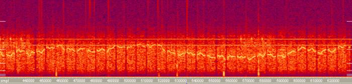
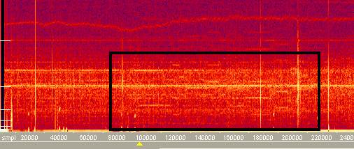
When looking at the spectrum versus time diagram below (it's even better if you listen), you see a whistle signal with much lower intensity during the pause times, which looks (and sounds) like the answer of another, more distant station.
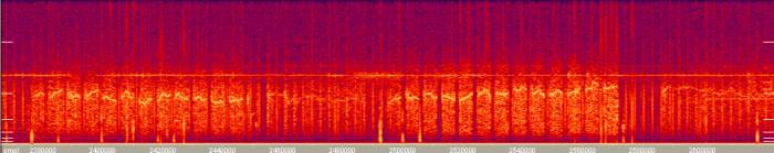
Figure: Two examples for answers of a distant station during the pauses.
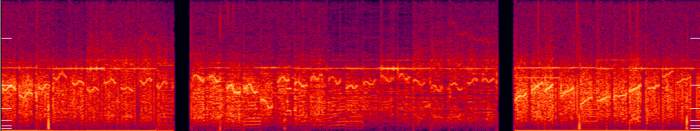
Another interesting part of the whistler signal is its beginning. The figure below shows the beginning of a transmission. On the left in the diagram, you can see that the transmission starts with a sequence of tones which are much shorter than the whistling itself and which have no background noise. The sound is very characteristic with a kind of stumbling beat, if you compare it to musical notes.
Each whistler transmission is characterized by such an introduction and until now, we could not find any matching between two of those sequences. If the whistling signal is really a kind of data transfer, then may be the introduction sequence is like a key for a certain code the signal is based on.
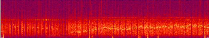
Figure: Introduction sequence of a whistling transmission (on the left)
Code or not?
The left part of the figure below shows inversions of the slash in the figure above. At the right part, the next character , a V-shaped line, can be recognized.
Figure: Negative slash and V-shaped character
For the V there also exists a clearly visible mirrored version, shown in the left part of the figure below. At the right part of the figure, a horizontal character is shown which means, that the frequency stays constant during the whistle.
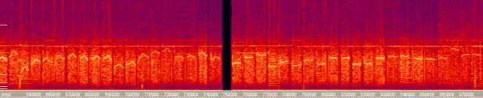
Figure: Mirrored V , horizontal line
The following characters are not quite clear. It cannot be excluded that they belong to one of the categories described above and are a little distorted by bad propagation conditions. It could also be that these characters are combinations of horizontal lines and positive or negative slashes.
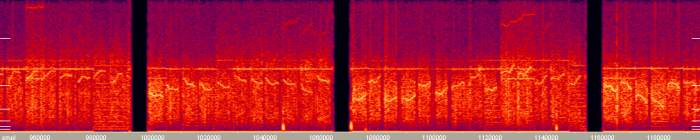
Figure:Are these characters four combinations of horizontal lines and slashes?
The different Y-axis-offsets of the characters are caused by the fact that they are picked randomly from different positions of a continuously mounting and falling time signal.
The different characters can not be recognized by only listening to the accelerated playback signal, because the characters are to short. But as the data transfer of each character lasts more than 20 to 30 seconds in real time, automatic decoding by some kind of electronic circuit should be possible (if it is data transfer at all).
Creation
of
the whistling signal
Needle printer signal
At the beginning of this article, we asked why some signals do suddenly appear, are present for some days, weeks or months and then disappear again for ever? This is not typical for machines used by housewives or hobby craftsmen. A typical example for this fact is the needle printer signal.
This signal appeared for the first time in December 2004 at Hürtgenwald with very high intensity and could be received uninterruptedly for a few days, disturbing all the other signals described in our parts I and II.
The figure below shows four elements of a repeating structure of 160 seconds (realtime). These structures sound exactly like an old fashioned needle printer, printing out one line.
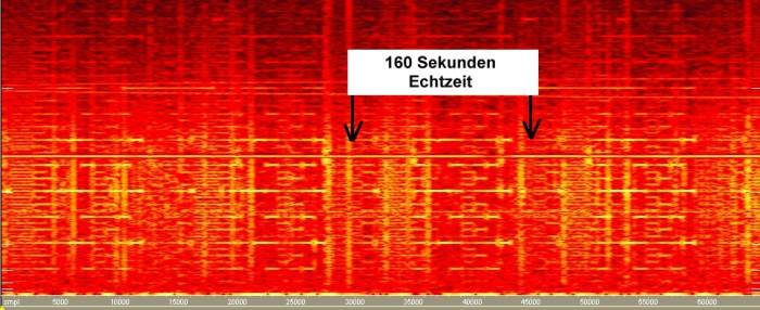
Figure: Spectrum of four of the continuously repeated elements of the needle printer (Text: 160 seconds realtime)
The figure below shows the corresponding time signal. The resolution is not high enough to visualize the complicated structure of one element.
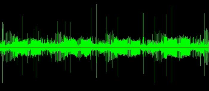
Figure: Time signal of the signal shown in the previous figure
The following two figures explain the structure of the elements in details:
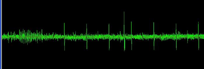
Figure: First section of a zoom of the time signal shown before: Each element starts with a series of pulses, which have a real time distance of 2.4 seconds. These distances are getting shorter
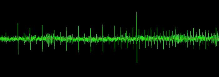
Figure: and shorter until their time distance is about 1,6 seconds. Then, the pulses are getting longer and shorter again alternatively (not shown in the figures).
The structure of the signal shows that it might be of an artificial origin, but if its really data transfer can not be said clearly. Inspite the fact that all elements sound equally, data transfer cannot be excluded: If you listen to a needle printer, it also seems that each printing of a line sounds equal though each time different characters are printed.
RTTY signal
What's quite normal in the range of commercial radio frequencies seems to be very strange in the ELF range: Below 16 Hz, we received signals which correspond exactly to the RTTY data transfer described above: Carriers who permanently jump between two or three frequencies of only a few Hz. In contrary to normal RTTY, one bit of the signals we received lasts many seconds or even minutes. Sending out only one word therefore would last a minute or more. If its really data transfer: Who would accept such low transfer rates and such a long transfer time if there would not be any advantage which pays for the patience?
On the other hand, facing the spectrum analysis of such signals, it's hard to find something different than data transfer as an explanation. The following signals not only show the simple type which consists of jumps between two fix frequencies but also the more complex multichannel signal type.
The first picture shows the analysis of a signal recorded at Hürtgenwald. Besides the signals in question, also the cow- and the goose signals are visible in the background. The signal is characterized by a lot of parallel spectral lines, changing their structure in time. The parts of the signal characterized by fast modulation appear a little bit blurred due to technical reasons, but if you are listining to it, you can clearly detect a kind of frequency modulation with the appropriate experience.
If you compare the RTTY-Signals in the figure below with the goose signals shown in the same figure, you will find out that the RTTY-signal is extended over a long time. In addition, the figure below only represents a short cut of a much more longer continuous RTTY-signal.
Figure: Multichannel RTTY-signal
The next figure shows the analysis of a recording made at Mariadorf. Besides the known goose signal (1 and 2), recorded synchroeously at Hürtgenwald (30 km away), you can see a kind of RTTY-signal with lower intensity (3). The signal is characterized by a permanent repeating of the following time symmetric pattern: Sinewave signal at lower frequency, sinewave signal at higher frequency, moulated signal, sinewave of higher frequency, sinewave at lower frequency.
Frame number four marks an also rather blurred section where frequency shiftings in positive and negative directions are happening around a center frequency of 12.5 Hz.
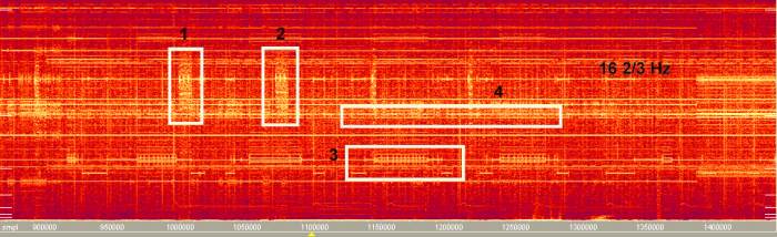
Figure: RTTY-signals in the frames number 3 and 4
The following figure shows the chronological sequence of the signal in frame number 3 at the previous figure:
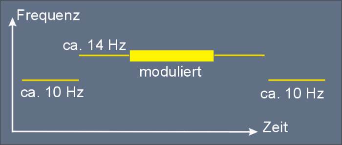
Figure: Schematical view of the spectrum of the modulated signal from the figure above (Zeit = time, Frequenz = frequency, moduliert = modulated, ca. = approximately)
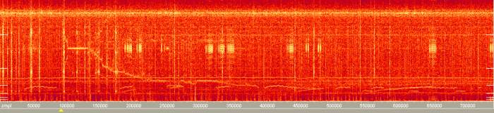
The following figure represents a recording made in september 2008 at the periphery of a small village (Biesingen), located 20 kilometers east from Saarbrücken, Germany at the countryside. The coil antenna was installed on a parking lot of a small solitary country hotel. The signal was registrated during the whole (holiday-) weekend. It also could be received in the hotel room (20 meters away from the parking area), but it had its maximum intensity at the parking lot.
The signal has a more simple structure than the ones shown at the previous figures as it only shifts between two or sometimes three frequencies. In addition, the signal is relatively high in its intensity and can be recognized clearly.
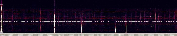
Figure:Signals from Biesingen near Saarbrücken, Germany
The shifting between two frequencies close to each other is clearly to see. Besides the two relatively strong main frequencies there seems to be a number of additional frequencies belonging to the signal. Due to the beackground noise its hard to give a precise judgement in this case.
The following figure shows a comparison between a day recording (left) and a night recording of the signal in question. In the night, the lower frequency seems having become higher.
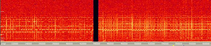
Figure: Recording during day (left) and during night at the same place at Biesingen
Commercial and military data transfer following this pattern is called FSK (Frequency Key Shifting) an still used for worldwide radio communication. If you play back the signal shown above (in acceleration mode), it sounds similar to the old morse code on shortwave.
The following signal was recorded in October 2008 at the Lake Bigge (Biggesee) 60 kilometers east of Cologne. In the figure you can see a number of parallel lines from nearly zero up to 25 Hz changing in their intensity. When playing back acceleratedly, the signal sounds exactly like a certain kind of multichannel FKS-Data transfer used on shortwave radio and reminds of the sound of a permanent chinese gong.
Figure: A complex multichannel data transfer?
Voice signal
Here some examples frequently repeated from day to day (pronounced in German language): Toooat, pieee, iglu, panic, sieben .
One of the longest sequences (recorded only one time) was:
Ju pi name ieee tieee (pronounced in German language). In English it would sound like: UP name ET.
The figure below shows the spectrum of the UP name ET sequence.
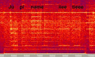
Figure:What does this mean?
The following figure shows a collection of cuts recorded at different days and glued together. When playing back, you hear words of vocals and consonants making no sense.
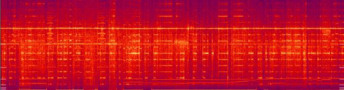
Figure: Collection of Voice-signals from different recordings
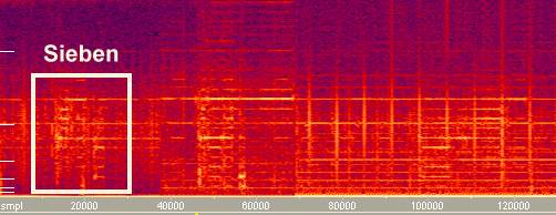
Figure: The German word Sieben (Figure 7) as spoken word (framed)
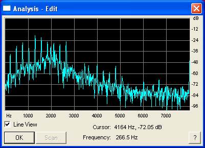
Figure: Spectral lines of the voice signal (the frequencies have to be divided by 160)
The FFT-spectrum (at a fixed time) shows in the lower frequency range (left) the regular distances of the voice signal spectrum lines. As the signal is multiplied in its frequency by 160, the frequency values shown in the diagram have to be divided by 160. The figure below shows the possible positions of the spectral lines (marked black) in a spectrum versus time diagram.
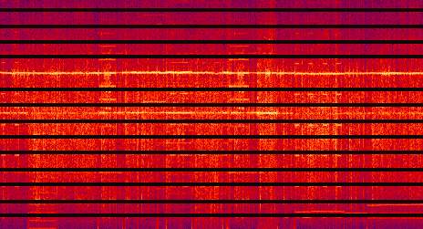
Figure:possible positions (black lines) of the voice signal harmonics (distances: 1,6 Hz)
Conclusion
The signals of type 2 therefore could also be signals which appear frequently at a certain place and which are typical fort this special location.
The fact, that at each new measurement location we found signals never detected before at different places, is of special interest. Some of these signals are similar to each other and therefore can be grouped together to one family .
The multitude of all the signals one more time puts the question of their origin: Are there really so many technical devices which create such a number of different signals? Why does each location has its own typical signals? Are they perhaps created by geological processes? This would not explain those obviously artificial structures found in the whistler-, the goose- or the RTTY-signals.
The optical quality of some the following screenshots is not so perfect because of the low intensity of the corresponding signals. Even in these cases you would get a good impression when hearing the sound of the recordings, played back acceleratedly. This is no wonder because the human ear inspite of all powerful software is still the best analyzer: Not before hearing the signal, we could identify the signal shown at the following screenshot as a typical needle-printer-signal, recorded at Allershausen, Germany.
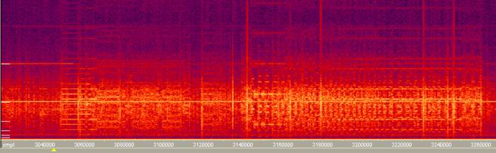
Figure: Another needle-printer-signal at Allershausen, Germany
Beep signal
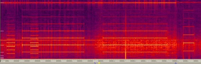
Figure: Three Beep-sounds. One at Hürtgenwald (left part) and two at Mariadorf (long and short sequences)
The spectrum of the beep sound (it really sounds a little like an alarm-beep signal of an electronic device) is comparable to the heartbeat signal, with the difference, that the spectral lines of the beep are much more expanded. It appears very rarely and could be registrated at different locations within Germany. The line at the upper margin of the picture was created by the 16 2/3 Hz supply current of the railway system. The short signal at the right margin is a little different in its frequency but sounds similar to the other ones.
Figure: Beep- signal at Bierbergen near Hildesheim, Germany
A second goose signal
Animal sounds
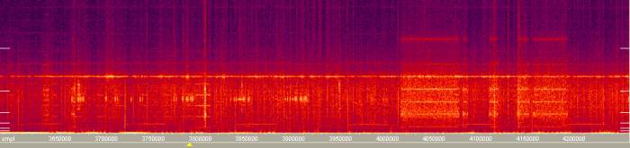
Figure:Animal sounds at Gerlingen (overview)
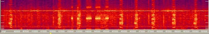
Figure:Animal sounds at Gerlingen (time-zoom)
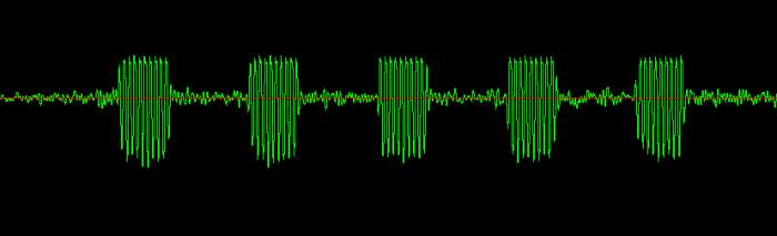
Figure:Animal sounds at Gerlingen (time signal at time-zoom)
Intermitting lines
At Hürtgenwald for example, an intermitting line of 25 Hz could be received nearly constantly for many years (picture above). As the 50 Hz Lowpass filter is already active in this frequency range, the intensity of the signal may even have been bigger than shown in the spectrum analysis.
In addition, 25 km away from this location, at the small village St. Jöris near Aachen, a similar signal (at 10 Hz) could be received. In spite of the big distance, the goose signal coming from Hürtgenwald can also clearly be seen.
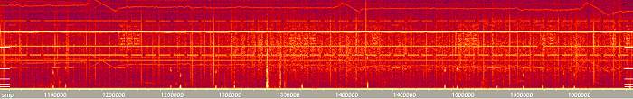
Figure: Intermitting line at St. Jöris near Aachen, Germany
Howling sounds
Ghost signal
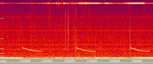
Sometimes, we found similar signals which differ from the fogey signals by a missing frequency shift (picture below).
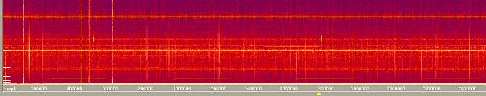
Figure: Signal at Zierenberg: Comparable to the fogey signal, but with constant frequency
Music
Foghorn
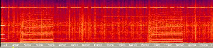
Figure:Foghorn Mariadorf
The picture below shows the differences between the spectrum of the foghorn (left) and the spectrum of the cow signal: The spectral lines of the foghorn are much more close to each other (in the frequency range). In addition, the mounting in the frequency range of the spectral lines at the beginning of the cow signal can not be found at the foghorn signal.
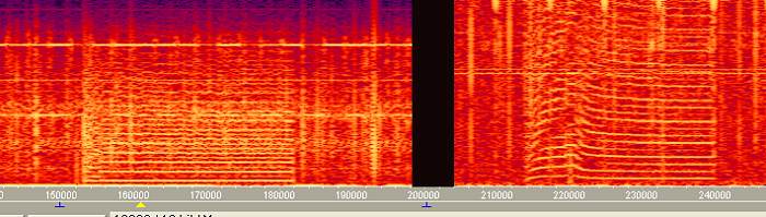
Figure: Comparison foghorn- and cow-signals.
Pan flute
Everyone may know the typical sound of a pan flute, when the player is shifting the instrument from right to left in front of his mouth: The listener hears a quick sequence of continuously mounting tones with sine character. At Bübigen near Saarbrücken in Germany, we recorded a sound similar to this in a house in the middle of a quiet housing area at the border of a forest. During the recording, the pan flute cycles repeated over the whole measurement period of four hours. The figure below shows two of those cycles which seem to be completely identical. Besides the typical pan flute sound with its arrow like spectrum, you can still recognize a sequence of bigger and longer frequency steps.
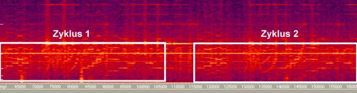
Figure: Pan flute at Bübingen
As the signal was not very strong, we highlighted the spectral lines in questions at the first cycle in the next figure.
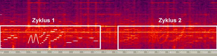
Figure: Pan flute at Bübingen with highlighted spectral lines
Irregular frequency
shifts
Figure: Squeal signal at Hürtgenwald
Slow frequency shifts
Figure: Slow frequency shifts
Finally: The authors are looking forward for any comment or important hint to this article.
In this case, please write to: contact@vlf.it
Author web page: http://www.subroutine.jimdo.com