MAGNETIC ANTENNA AND OBSERVATION OF TWEEKS
Tay Nguyen university, Vietnam
INTRODUCTION
Last year, I installed the AWESOME-VLF receiver from Stanford university with my research group. It is easy for setting up that receiver. I only read the guide document and installed it carefully, thus it ran well. But I don’t understand how its circuit work and how to calibrate the VLF receiver for recording the good signals. One day, I found the excellent website, www.vlf.it. I read some articles [1, 5, 7, 8] which give me ideas to design a VLF receiver.
This article
aims to present the some experiences about
installing the VLF receiver with the magnetic
antenna, and capturing the tweeks at a low-latitude
station in Tay Nguyen University, Viet Nam (12.650 N; 108.020 E).
SETTING UP THE VLF RECEIVER
|
|
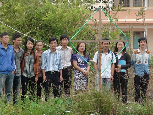
We assembled the square loop with a
side of about 1 m (Fig.1). The antenna has 14 turns of aluminum
wire of 1.2 mm2 section, the total resistance of
1,2 ohms and its inductance value of 0,748 mH. The wires are wrapped by the aluminum foil. This shield is connected to the ground with the parallel 4 rods. Everything is covered with the plastic tube. The loop is installed near a small beautiful lake at Tay Nguyen university where is relative quiet. |
b) THE AMPLIFIER
We modified the Paul’s circuit to be suitable to our local station. The amplifier has two stages, and we add the low band filter between the two stages for decreasing the city noise.
The op-amp LT1028 is used for the first
stage, which has ultralow noise precision with 0.85nV/![]() 1kHz noise and
high speed specifications with 75 MHz gain-bandwidth.
The LT1028’s voltage noise is less than the noise of a
50Ω resistor. Therefore, even in very low source
impedance transducer, the LT1028’s contribution to total
system noise will be inappreciable.
1kHz noise and
high speed specifications with 75 MHz gain-bandwidth.
The LT1028’s voltage noise is less than the noise of a
50Ω resistor. Therefore, even in very low source
impedance transducer, the LT1028’s contribution to total
system noise will be inappreciable.
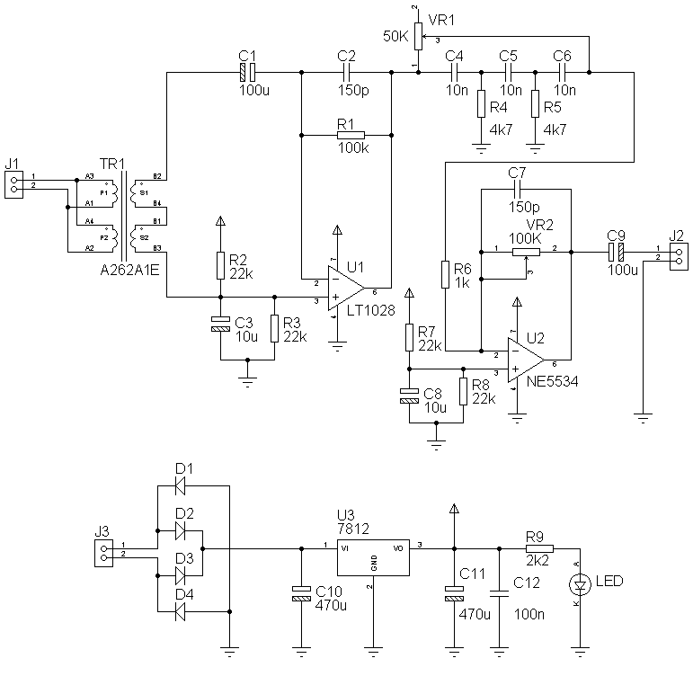
Figure 2. The circuit
diagram of pre-amplifier
The
NE5534 is used for the second stage, which is not the
best op-amp for our project. But it is accepted because
the gain is stable. The variable resistor (VR2) is used
to be the negative feedback resistor and to adjust the
gain.
Our observation is near the broadcasting station, so we used the capacitors C2 and C7 with 150pF which can limit the gain at high frequency and may be necessary to prevent oscillation. They also reject the HF interferences.
The amplifier board is wrapped with the metal box to decrease the noise (Fig. 3).
For the loop transformer, we used the audio transformer (A262A1E) which has winding ratio 12.6: 1, 3.75 ohm primary windings and 150 ohm secondary winding. Jack J1 connects between the transformer and the antenna. The ground isolation transformer (A262A7E) is used with 600 ohm to 600 ohm, it is common for audio applications to break ground hum loops. It is inserted between the jack J2 and the Soundcard (Realtek HD Audio) on board of PC. We tried to find a relative quiet place where is far away form the building house, so the cable length must be so long with 200 m.
The DC supply adjustable is used for power supply. We also used the bridge of diodes D1 – D4 (1N4007) to avoid the reverse bias, and used IC 7812 for the constant voltage of the amplifier.
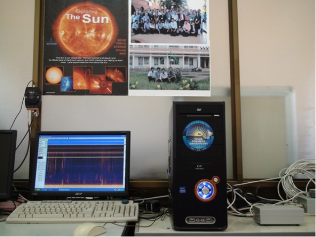
Figure 4. The PC for recording the VLF data during the day and night
OBSERVATION OF TWEEKS
1) BACKGROUND
Tweeks are the electromagnetic pulses with the extremely low frequency (3-3000 Hz) and very low frequency (3-30 kHz) bands which are emitted by lightning discharge with frequency dispersion. These electromagnetic pulses are reflected in the Earth-Ionosphere waveguide (EIWG) and propagate thousands of kilometers with the cut-off frequency of about 1.8 kHz. The waves are recorded by the receiver and heard as “tweet” in the literature [9].
The electron density was estimated using the relationship [3]:
![]() (1)
(1)
where fc is the cut-off frequency of the wave guide
Therefore, the cutoff frequency for nth mode is given by:
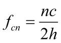 (2)
(2)
Where c is the speed of light in the vacuum and h is the height of EIWG.
Group velocity v for nth mode is given by [4]:
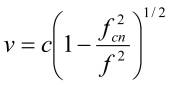 (3)
(3)
We have
 (4)
(4)
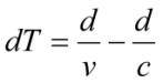
Therefore, the distance propagated in waveguide is given by [1]:
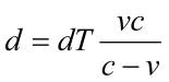 (5)
(5)
dT is the dispersion time for tweek which can be calculated from the spectrogram fcn is cutoff frequency for the nth mode and f is the frequency of the wave.
The reflection height h is obtained by the first mode cutoff frequency fc as follows:
 (6)
(6)
Therefore, using tweek atmospherics, we can determine the electron density (Equation 1), the propagation distance from the lightning source to the observation site (Equation 5) and the night time reflection height (Equation 6).
2) ANALYSIS OF TWEEKS
We captured many tweeks in 28 October, 2012. The broadband data were recorded by Spectrum Lab with the wave files. They were recorded for 60 seconds at every hour, from 17:00 LT to 05:00 LT. We used the Sonic Visualiser software to record t, tc, f, fnc for estimating the dT, v , h, d, Ne.
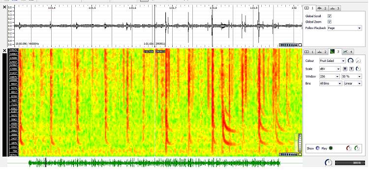
For showing the tweeks so clearly on Spectrograph, choose the 256 FFT for window and the fruit Salad for colour (Fig. 6).
 a) b)
a) b)
 c)
d)
c)
d)
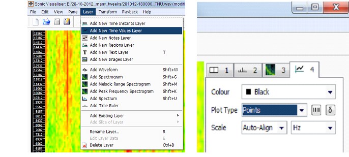
On the menu bar, click Layer and choose Add New
Time Values Layer, then select
the Points for the plot type. Note that, we
must select the Hz unit on the right box of the Scale
(Fig. 7 a,b).
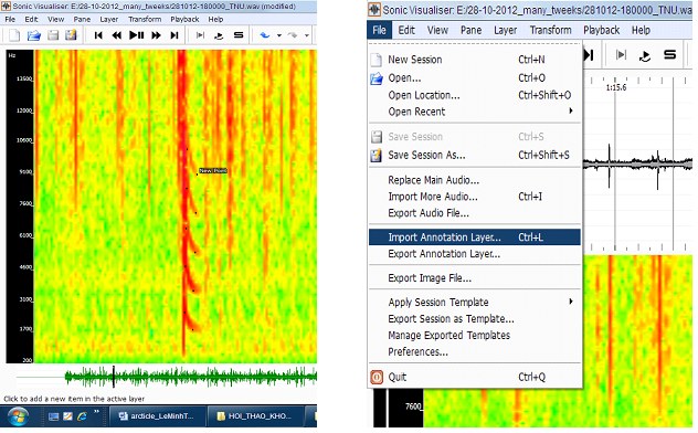
The first, click the mouse
to retouch the points on the first vertical line for
recoding the frequency (f). After that, click to
retouch the points on the tails of hooks for capturing
the cut-off frequency with different modes. Finally,
select File Export
Annotation Layer for producing
the csv file, and then make the spreadsheet for
analyzing the data (Fig 7 c,d).
3) RESULTS AND DISCUSSION
The time of occurrence of tweeks were classified into two periods pre-midnight (17:00 – 23:00 LT) and post-midnight (23:00 – 05:00 LT). Table 1 shows that the percentage of the occurrence of tweeks in the pre-midnight (63.65%) was higher than in the post-midnight (36.35%). The tweeks from 2nd harmonics to 4th harmonics occurred more often than the tweeks with different harmonics. The tweeks with 8th modes have the lowest percentage and they had not been found in the post-midnight.
Table 1. Occurrence of tweeks in period 28 October, 2012
-
Period of night
Total number
of tweeks
Percentage of occurrence
Number of Tweeks with different modes
1st
2nd
3rd
4th
5th
6th
7th
8th
Pre-midnight
366
63.65
3
80
125
103
34
8
8
5
Post-midnight
209
36.35
7
62
60
47
18
9
6
0
Total
575
100.00
1.74
24.70
32.17
26.09
9.04
2.96
2.43
0.87
Table 2. The cut – off frequency, mean frequency, reflection height, propagation distance and electron density calculated from tweek sferics.
-
Spectrogram
mode number
fcn (Hz)
fcn/n
(Hz)
h (km)
d (km)
Ne (el/cm3)
a
1
2
2007.64
4167.01
2007.64
2083.51
74.71
71.99
5605.65
3979.67
33.33
34.59
b
1
2
3
2122.48
3885.92
5692.38
2122.48
1942.96
1897.46
70.67
77.20
79.05
1869.37
2348.27
3398.84
35.23
32.25
31.50
c
1
2
3
4
1824.1
3743.45
5606.35
7130.55
1824.10
1871.73
1868.78
1782.64
82.23
80.14
80.27
84.14
2466.56
1601.69
986.91
1344.42
30.28
31.07
31.02
29.59
d
1
2
3
4
5
6
7
8
1846.99
3634.68
5422.36
7146.2
8997.73
10721.6
12700.8
14296.9
1846.99
1817.34
1807.45
1786.55
1799.55
1786.93
1814.40
1787.11
81.21
82.54
82.99
83.96
83.35
83.94
82.67
83.93
2526.46
2326.60
1758.31
1598.66
1470.05
1522.22
1194.16
1175.31
30.66
30.17
30.00
29.66
29.87
29.66
30.12
29.67
Table 2 shows the mode numbers, cut-off frequency ‘fnc’, mean frequency ‘fnc/n’, ionospheric reflection heights ‘h’, propagation distance ‘d’ and electron density ‘Ne’ estimated from the tweeks shown in spectrograms (a – d) of Fig 8. We can see that the mean frequency with higher modes decreases slowly. The height is calculated for the different modes of tweeks, which increases with increase in n and varies from 71,99 km to 83,96 km. This shows that higher harmonics penetrate deeper into lower D ionosphere region. We also found that the electron density varies in range of 29.66 – 34.59 el/cm3.
 |
 |
About 575 tweeks obtained during the night in 28, October were analyzed and the average reflection height h, the average electron density Ne were plotted for different modes n = 1- 4. The variation of h and Ne are shown by the dash line with circles (right hand scale), the solid line with diamonds (left hand scale), respectively. Fig. 9 shows that the h and Ne dramatically change during sunset (17:00-19:00 LT), midnight (22:00 – 00:00 LT) and sunrise (4:00-5:00LT). Both of them vary with the same shape, and change symmetrically, but they vary slightly in n = 4. The h from 2th to 4th modes shows similar variation with maximum at around 23:00 LT. Similar the case, Kumar et. al. (2008) found that the maximum value of heights occurred at around 1:00 LT at Suva (18.20 S, 178.30 E) [2]. The Ne decreases and varies in range of 72.09 – 89.07 km as the h increases and varies in range of 28.16 – 34.74 el/cm3. The results of h at our site approximate to those of the h (73 – 87 km) at Universiti Kebangsaan Malaysia (2,550 N, 101.460 E) [6].
|
|
Therefore, the h and Ne values depend on the cut-off frequency and this indicates that the upper boundary of the EIWG is not sharp bounded and homogeneous.The propagation distance ‘d’ is calculated by using equation (5), which is presented in Table 2, and the occurrence rate of tweeks of 28, October as a function of propagation distance is shown in Fig. 10. We can see that the d varies with mode number and varies from 300km to 16000 km. the propagation distances of tweeks with higher mode are shorter than those of tweeks with lower mode. About 81.6 % of tweeks have the d in range of 1000 – 7000 km. The maximum percentage (18.7%) of occurrence rate of tweeks has the range of 2000 – 4000 km. |
CONCLUSIONS
Using the simple magnetic antenna, the amplifier and soundcard of PC, we can record many tweek sferics clearly. The parameters of EIWG were estimated from the tweek sferics obtained during the local night in 28, October, 2012. The reflection height of EIWG and the electron density of D ionosphere region vary in range of 72.09 – 89.07 km and 28.16 – 34.74 el/cm3, respectively. The tweeks with higher modes come from nearby sources and most of tweeks from 2nd to 4th harmonics occurred.
ACKNOWLEDGMENT
We thank Renato for many help and Paul for giving the amplifier circuit. We would also like to thank Jean Claude and Torsten for sharing many experiences about installing VLF receiver and analyzing the tweek data.
REFERENCES
[1] Alves Thierry (2003), “Simple Earth-Ionosphere waveguide calculation”, www.vlf.it
[2] Kumar, S., A. Kishore, and V. Ramachandran (2008), “Higher harmonic tweeks sferics observed at low latitude: 5estimation of VLF reflection height and tweek propagation distance”, Ann. Geophys., 26, pp 1451 – 1459.
[3] Ohya, H., M. Nishino, Y. Muryama and K. Igarashi (2003), Equivalent electron densities at reflection heights of tweek atmospherics in the low-middle latitude D-region ionosphere, Earth Planets Space, 55, pp 627-635.
[4] Outsu, J. (1960), “Numerical study of tweeks based on wave-guide mode theory,” J. Proc. Res. Inst. Atmos Nagoya University Japan, 7, 1960, 58-71.
[5] Renato Romero and Marco Bruno (2000), “An easy VLF Loop”, www.vlf.it
[6] Shariff, K.K.M., M. M. Salut, M. Abdullah, K. L. Graf (2011), “Investigation of The D-Region Ionosphere Characteristics Using Tweek Atmospherics at Low Latitudes”, Proceeding of the 2011 IEEE International Conference on Space Science and Communication, Penang, Malaysia.
[7] Torsten Heer (2010), “The B3CKS VLF - antenna project”, www.vlf.it
[8] Wilfried Fritz (2012), “A very simple VLF Pocket receiver”, www.vlf.it
[9] Yamashita. M (1978), Propagation of tweek atmospherics, J. Atmos. Terr. Phys., 40, 151–156.