An air core loop able to receive Schumann resonances can easily be constructed, as presented in the article A Minimal ELF Loop Receiver in this web site (www.vlf.it/minimal/minimal.htm). Its characterization and use in unattended operations cannot always be that easy: lets see how to face some troubles in activating a serious non stop RDF monitoring system.
Minimal Loop
characterization
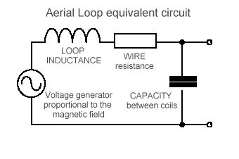
From the electronic literature we know that a real
loop can be considered as a result of three components: an inductance,
a resistance and a capacitance.
The resistance works in series to the inductance and is caused by copper wire resistance: it determines the low corner frequency of the loop, reducing performances and introducing thermal noise. From here, we can easily assume that a loop with a low resistance works much better, then more copper weight we use, better performance we can obtain.
The capacity instead stays in parallel to the inductance-resistance series: it represents the distributed capacity between the inductance coils. It reduces the performances at higher frequencies making the loop self-resonate. The knowledge of exact values of these components can be very useful when we want to project a proper amplifier.
Resistance is easy to be measured: a simple analogic tester or a digital multimeter can be used to do that, but inductance and capacitance are not that easy to determine. We can not use cheap portable LC testers because they measure at 1 kHz (the minimal ELF loop can be over the self-resonating frequency) and they cant separate inductance from capacitance (these cheap instruments want only see a single parameter: L or C). Therefore, how can we do that?
An easy way comes by observing where the loop self-resonates. We need an audio generator: or a function generator or simply an audio card. Putting a 100 kOhm resistance in series with this generator we obtain an high impedance generator. Then we connect this high impedance source to our loop, moving frequency from few Hz to some kHz, and observing where the voltage to the loop terminal reaches the maximal value. This is the self resonating frequency. To read this voltage, we need an oscilloscope, or a high impedance meter. We can use the audio card as well, by putting in series another 10 kOhm resistance.
In order to complete the operation, we have to put
an external capacitance of some tens of nF (for example 30 nF) and repeat
the measure, obtaining so a second resonating frequency.
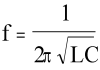
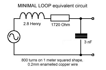
We can now apply the measured value to the resonating formula (two equations with two unknown parameters) and we can calculate the C and L real value by the minimal loop. The minimal loop presented in this web site appears as shown here:
How the minimal loop reacts to a magnetic field variation
To confirm how the minimal loop reacts in frequency to a magnetic field, we generate a constant field with a link loop: 10 turns loop wounded under the minimal loop, and a function generator used with 50 Ohm impedance output and with 10 kOhm resistance in series. This configuration allows maintain a constant current in the link loop also varying the frequency, and then it allows generate a constant field at different frequencies. Current frequency value has been verified frequency by frequency with an oscilloscope.
We now generate signal from 10 Hz to 10 kHz and
we are able to read with in an oscilloscope the output voltage on the minimal
loop, leaved electrically open; then we can so do the same by terminating
the minimal loop on a 27 Ohm resistance the voltage on the resistance.
The first measure shows how the minimal loop works
in voltage (see the blue trace, named voltage output), and the second
one how it works in current (see at the red
line, named Current output).
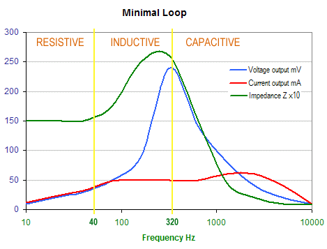
We can see two interesting different attitudes, that confirm the validity of the equivalent circuit.
If we use the minimal loop terminated on a high impedance preamplifier (blue line), we have the maximum voltage response at resonating frequency at 320 Hz, after that the loop decreases its performance; frequency response is not linear but it regularly increases with frequency up to the resonating frequency.
If we use the minimal loop terminated on a low impedance preamplifier, as reported in the virtual ground circuit at http://www.vlf.it/minimal/minimal.htm , we have a signal output proportional to the current: frequency response is linear from low frequency corner up to 10 kHz because the parasite capacitance is shorted by low impedance. We can see as the minimal loop also works in higher frequency than self resonance one.
We also can recognize the three different frequency ranges:
Mechanical stabilization
Lets return to the practical problem. One of the worse troubles we find in using the minimal loop is the microphone effect: a loop millimetric mechanical oscillation produces a big interference, this is because the antenna works fitted in the terrestrial magnetic field. Since we cant turn off the heart magnetic field, we need to make the loop perfectly stable.
Ive tested different expedients: with elastic ropes (the ones used in the roof baggage racks car), with wood poles ; they work well in weather good conditions, but as soon as the strong wind starts to blow, the whole system resonates mechanically, making useless every attempt reception. Another solution can be an underground hole where to bury the loop, but the loop measures (1m x 1m) are not minimal enough: a pit of one meter is not a trick. How to lock it, then?
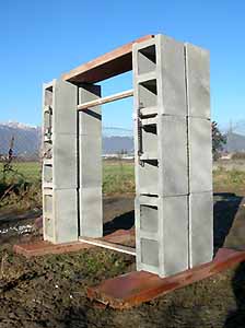
A minimal loop (1m x 1m) locked in a cement blocks. The preamplifier in stereo version, realized with two OP27, connected in virtual ground configuration
This one, showed in the picture, is a very low cost expedient, but it works very well: the minimal loop is locked in cement blocks. They cost 2 € and weight 10 kg each one: to stabilize a single loop, we have enough of 12 blocks, for a total of 120 kg (and you can now understand why it effectively stabilizes the loop).
A minimal loop, now locked in cement blocks, is able to work also for unattended operation for long time monitoring. We can use it as reliable tool to see submarine communications, Schumann resonances, magnetic ELF signals caused by solar activity and all the other strange signals we can find there
Direction finding in ELF
What does it happen if we make a second loop, placed orthogonally to the first one, on the same frequency range? We can do a RDF extremely low frequency monitoring: looking the direction of the submarine signals, or tracing the directional component of the Schumann resonances.
The software SpectrumLab, as for the other VLF examples
reported in the DL4YHF web site, can make directional spectrograms also
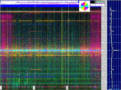
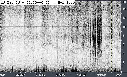
for ELF frequencies. Here below is shown an example of 1 hour reception.
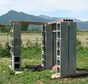
Two minimal
loop in orthogonal position (East-west and North-South), locked in a cement
block.
The spectrogram,
where Schumann resonaces are evident, have been acquired with this system.
We can see some weak changes in the noise background, otherwise they are not detectable with a commune spectrogram. I think this can be one of the most powerful ways to investigate the seismic precursors, and we are able to know if before an earthquake an ELF radio emission is detectable, and the direction from which it comes.
Unattended operation
Every serious monitoring needs a long time operation and a big data quantity: if we are looking to radio seismic precursor, we need to think of unattended operations, for long time and with automatic saving data system. SpectrumLab realizes these fundamental features with a very simple command string.
A good trick to optimize the picture saving is to obtain the best output from a spectrogram: if we use a FFT resolution of 0.1 Hz we can obtain the best compromise by putting the scroll time at 10 seconds. If we set a shorter time, we stretch the picture with the same data, wasting so pixels; if we set a longer time scroll, we loose data. We can control this setting in the Configuration and Display Control windows, in the FFT properties: the overlap from scroll interval must be from -20 to + 20%.
The picture can contain data about time and frequency, it can be very helpful in a second time to control the collected spectrograms. Here there is a simple sentence to type in the screen capture options to put date, time and frequency range in the spectrogram:
"Date="+str("YYYY-MM-DD",now)+"
Time="+str("hh:mm",now)
"Freq=
"+str("###0.#",water.f_min)+"..."+str("###0.#",water.f_max)+" Hz"
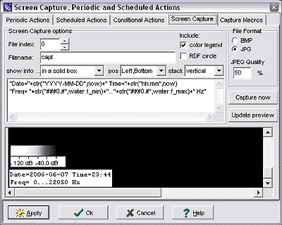
Here sentence to put in the Periodic Actions macros: it allows spectrograms capture (in jpg format) and the received data saving (as wave file):
capture(str("DDMMMYY-hhmm",now)+"_rdf.jpg")
wave.record(str("DDMMMYY-hhmm",now)+"_rdf.wav")
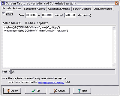
This produces an automatic archive of wave files and jpg pictures, for a complete log of the ELF activity. Before starting with an automatic wave file saving do not forget to activate the wave file decimation function. The command is in configuration and display controls, inside the wave file folder: you have to cross the decimate saved audio files and put a proper value. If you are monitoring the 0-100 Hz frequency range a good value can be 230 sample/sec: saved wave files will contain frequency between 0 to 115 Hz (sampling rate /2), and will be of (relatively) small dimensions.
An ELF whistler, or something that seems to be that, captured during unattended operations: it's placed on the first Schumann resonance and is 15 minutes long. This picture has been obtained post processing the wave file with Cool Edit.
Two channels sampled at 230 samples/sec produce a wave file of about 12 Mb every 4 hours: saving a jpg picture every 4 hours we have a complete daily log in about 62 Mb, wave files and jpg pictures. Archiving data on a DVD we can save two months on a single disk.
Last but not least, do not forget to set in
your PC BIOS the correct start-up: activating the start with last working
condition setting, when the power returns after a blackout, the PC turns
it on automatically. If a link of SpectrumLab executable
has been put in automatic execution folder, the PC starts automatically
to log the activity.
Conclusions
This cheap setup, composed by two minimal loops,
two simply preamplifiers and a single audio card managed by SpectrumLab
software, can allow the realization of a professional ELF monitoring station.
Some features, once available only with professional devices, can belong
now to everyone: in my setup an old 400 MHz Pentium processor manages two
audio cards that work together; 4 channels are available for RDF magnetic
activity, electric field and a geophone, with automatic saving of pictures
and wave signals. Sometimes the power turns off, but thats not a problem:
when the power returns the station starts to work automatically.