INTRODUCTION
When this article was begun, the idea was simply to summarize the results of a work that was published nearly 40 years ago by Maxwell and Stone1 who reviewed their measurements of natural ELF and VLF noise in an IEEE journal. Recently some newer data by Chrissan and Fraser-Smith2 has been found that both supports and expands the older data. In short, both papers data show an average noise density of about 1 picoTesla per root-Hz at 1 Hz frequency decreasing at about 10 dB per decade (of frequency) to about 0.1 pT per root-Hz at 100 Hz. At this point the rate of decrease is about 15 to 20 dB per decade up to about 2 kHz. Between 2 and 7 kHz there is a variable minimum, or dip, in the noise curve which then rises sharply to a maximum at about 9 to 10 kHz. Above 10 kHz the noise decreases at the rate of about 20 dB per decade up to the 100 kHz upper frequency limit of the studies. The number of papers focused on ELF/VLF propagation has increased greatly since the 1990s. The first mass of papers, from the cold-war era, was sponsored directly or indirectly by the desire to communicate reliably with deeply submerged submarines. The more recent interest is probably driven by the desire to predict natural phenomena, mostly disastrous phenomena such as earthquakes, volcanic eruptions, large-scale storms, and the like.
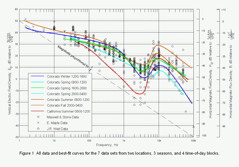
The intent of this article is to provide a basis for amateur research by reviewing some of the work done regarding the ELF/VLF noise floor, and, hopefully, suggest some directions for that research. Knowing what the natural noise level is will allow us to know when our receivers are "hearing" environmental noise and not their own "front-end" noise, and should suggest some areas for individual and networked, or cooperative research. Figure 1, taken from Maxwell and Stone, illustrates that the noise spectral density is affected by many variables. All of the data from their 1963 paper from seven different measurement series is plotted on this single graphic. These data were measured at sites isolated from power line and industrial noise in Colorado and in central California and span all seasons of the year and time blocks in the daily diurnal cycle. Figure 2 is data from Chrissan and Fraser-Smith and shows only data recorded at a site near Stanford University about 200 km north of the Maxwell and Stone site. This graph shows monthly averages of noise spectral density, and is generally consistent with the earlier Maxwell and Stone data with a few exceptions that we will discuss later.
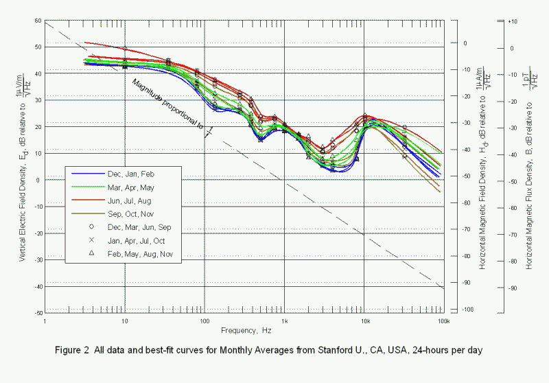
Chrissan and Fraser-Smith placed identical radiometers (noise measuring systems) at four locations representing mid and high latitudes in both northern and southern hemispheres. The data were collected contiguously from 1985/86 through 1993/94. Their paper is a presentation of the data averaged over months of the year for each station, and for four-hour time blocks that are averaged for each month of the year for each station. These data have been reformatted for plots of noise spectral density versus frequency. Only the data measured at Stanford is included in this article because it represents a mid-latitude northern hemisphere location.
The frames for all noise spectral density graphs in this article are the same to facilitate comparison. The vertical axes are calibrated in electric-field intensity (E), magnetic-field intensity (H), and magnetic-flux density (B) units. The use of both electric-field and magnetic-field units to describe the same curve implies that both E and H are related (bold font represents vector quantities). Maxwell and Stone found, by direct measurement, that the electric field was vertically polarized and the magnetic field was horizontally polarized. Further, the ratio E/H, using simultaneously-measured magnitudes of E and H, was very close to 120p (or 377) ohms, which is the impedance of free space. The polarization and 120p-ohm ratio implies that the noise fields are truly propagating plane waves and are not quasi-static or near-field quantities. The exception to this rule is fields produced by nearby storms and most man-made (cultural) noise .
Also drawn on each graph is a hatched line with a slope of -20 dB per decade of frequency. Many natural processes, including thermal noise generation, produce a noise power spectral distribution such that each octave, or decade, or any geometric progression of frequency contains the same amount of total noise power. This is equivalent to stating that noise power spectral density is proportional to 1/f. The hatched line clearly does not represent the noise spectral density at frequencies below about 20 kHz. Notice that in the highest decade of frequency all the curves begin to approximate the slope of the line. This observation illustrates the great variability in the spectral characteristics of both noise sources and the propagation medium. (Note: if the Y-axis scales were in units of power, the slope would be -3 dB/octave, -10 dB/decade, etc.)
Since the Maxwell and Stone data were acquired seasonally and monthly at widely separated locations, and different times in the diurnal (daily) cycle the plotted curves for each data series differ somewhat. The Chrissan and Fraser-Smith data, in Figure 2, are averaged over the entire diurnal cycle, but show month-to-month variations. It is clear that seasonal, diurnal, and geographic factors all affect the local noise spectrum. It is also clear that some other factors may be at work as well. Well discuss some of these later. It should be noted that the authors (and their co-contributors) avoided measurements at the Schumann resonance frequencies as their objective was to characterize the noise sources and the propagation medium, and not well-known second-order effects such as resonances.
Writing this article has been like climbing a tree where one encounters ever more specialized branches. We will try to keep this on a "readable" level and provide some quantitative "benchmark" data that can be used to determine how well your receiving apparatus performs in a noisy environment. When we consider the causes of variations in the noise spectrum, you may wish to perform some experiments to verify the data and, perhaps, add some new observations. All-in-all, the objective of this article is three-fold:
2) To challenge Open Lab readers to expand, or correct this information, and
3) To suggest some areas of research that can be performed at the amateur level with equipment and facilities available to all of us.
ULF/ELF/VLF NATURAL NOISE
Natural noise in the lowest-frequency portion of the electromagnetic spectrum is dominated by lightning flashes all over the world. An average of 2000 storms exist worldwide at any time producing about 100 lightning strokes per second. The noise sensed at your location is influenced by the propagation path between you and the location of each lightning stroke. The recent discovery of direct and indirect lightning-related phenomena ("trimpis", "red sprites", etc.) occurring between storm cloud tops and the lower ionosphere (30 to 90 km) adds another, possibly significant, source to ELF and VLF noise and discrete, spheric-like events. In auroral regions, "polar chorus" and "auroral hiss", excited by high-energy solar protons may dominate the ELF band. Less powerful sources of ELF and VLF noise include tornadoes, volcanic eruptions, dust storms, and probably earthquakes. Prediction of the latter by ELF signals has been a priority for a number of researchers and is an area where amateurs could contribute in data collection efforts. The summation of signals propagating in the earth-ionosphere duct produces the relatively continuous noise level that is punctuated by spheric bursts. Barr, et al3, (ELF and VLF Radio Waves) is an excellent summary of ELF and VLF research over the last 50 years, and is the source of much of the information in this article. (You may be able to find this paper as a free download on the internet, although my copy was a 30 USD .pdf file from Science Direct.)
LIGHTNING
There are many phenomena contributing to the noise spectrum, but lightning flashes are by far the dominant source. Anyone interested in other sources (auroral phenomena due to solar particle bombardment, volcanic eruptions, hurricanes/typhoons, dust storms, etc.) can easily find a wealth of material on the internet. Keywords "vlf radio noise" will "Google-up" enough references to keep you busy for a long time. Lightning has enough variants to warrant a series of articles all to itself. Briefly, a lightning discharge consists of three main parts. A series of leaders, each about a m sec in duration with peak current about 300 amps and each leader being separated from the next by 25 to 100 m secs occur over a period of about a msec. The leaders ionize a channel for the return stroke or main discharge which lasts about 100 m sec and has peak current of the order 30 kilo amps. Last is the slow tail, an exponentially decaying current initially of several hundred amps that persists for about 0.5 sec. Each of the three parts produces radiating energy in different parts of the spectrum. The leaders, being the shortest, produce energy in the low LF range, generally above 30 kHz. The main discharge produces a large radiating pulse with energy centered broadly around 10 kHz. The slow tail, of course, being long, is one of the principal sources of ELF noise.
A large majority of observed lightning strokes are cloud-to-ground (CG). The leaders produce a negatively charged channel that the main return stroke neutralizes. CG discharges, being largely vertical currents, efficiently couple energy to the earth-ionosphere duct, which favors vertically polarized radiation. Intra-cloud (IC) discharges are less well known, primarily because they are visually masked by cloud. IC discharge components are mostly horizontal, which does not couple well to the propagation medium. However, IC paths are considerably longer than CG paths, and the vertical portion of an IC flash path is about 1/3 of its total length. Thus about 1/3 of the total IC energy does couple to the medium with the result that both IC and CG flashes contribute about the same noise energy. That is, the current-distance moments in the vertical direction are about the same.
About 2/3 of the total lightning strokes worldwide occur in the tropics of Central and South America and South-Eastern Asia. Lightning storms in mid latitudes occur generally during the summer months. Hence, to some degree, lightning activity migrates between northern and southern hemispheres semi-annually.
The contributions to the total natural noise spectrum of the three lightning components are not equal in magnitude, and centers of lightning activity world wide tend to migrate seasonally. Each of these source factors affects the temporal variability and non-uniformity of the noise spectrum up to at least the LF region.
PROPAGATION
The second factor affecting the ELF/VLF noise spectrum is the propagation medium. The earths ionosphere is familiar to all radio amateurs and short-wave listeners. However, the familiar HF bands are affected, or rather, enabled, by the F1 and F2 layers with some influence by the E and sporadic E layers. HF generally penetrates the lower, less densely ionized regions. The D region, which borders the neutral atmosphere, is the layer that appears highly magnetically conductive to LF and lower frequencies. The D region is primarily a daytime phenomenon. At MF (medium frequency) the D region is an efficient attenuator (because of energy absorption due to ion collision and recombination) which explains why distant MF broadcast stations can often be received only at night when the D region effectively disappears and E region reflectivity comes into play. At VLF and below, the D region is the top of a waveguide duct during daylight hours. The effective height of the waveguide varies with the appearance and disappearance of the D region on a diurnal basis. (Note: we use diurnal because it refers to night and day rather than sidereal which refers to star passage.)
Davies, in Chapter 9 of his book Ionospheric Radio Propagation4 develops both ray theory and waveguide theory of LF and VLF propagation. Ray theory is not very useful because VLF wavelengths are of the same order as the height of the D region. However, it helps explain "the diurnal change D j in phase as due to changes in the height D h of a fictitious reflecting layer." Davies uses the term "fictitious" because a sharply defined reflecting layer (the D or E region) does not exist. The lower ionosphere is a diffuse mass of neutral molecules, positive ions and free electrons that appears below the E region during the daylight hours. However, its appearance to a wave of a particular frequency and angle of incidence is that of a well-defined reflector.
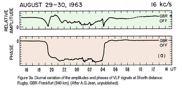
The phase change of a stable VLF transmitter as received at a distant location resembles a trapezoid when plotted against time over a diurnal period. The edges of the trapezoid coincide with the mid-path sunrise and sunset. Short paths show steep edges, while long paths show slowly changing edges. The phase of the received signal is much more stable during daylight hours when the D region is well formed, but is quite variable during hours of darkness when the D region is, for all intents, gone and the reflecting layer is due to E and sporadic E ionization. Figure 3, taken from Davies, p 424, illustrates this effect for a short path (upper diagram) and a long path (lower diagram). Although "noise" has no meaningful phase, the change of effective height during the diurnal cycle (the cause of phase and amplitude change in a coherent signal) modifies the propagation characteristics of the earth-ionosphere waveguide. A waveguide supports propagation mode-models rather than a ray-model. At frequencies above the waveguide cutoff frequency (below which propagation cannot occur) one or more modes are possible at any particular frequency. When the dimensions of the waveguide become smaller, fewer and fewer modes can be supported. When a propagation mode change occurs because of a discontinuity in the waveguide size (ionospheric height), the path "sees" a change in attenuation and phase characteristics. Since the bottom of the ionosphere, globally, varies greatly, the paths from sources worldwide to your receiver vary as well. Generally, the waveguide characteristics near your location will dominate, as can be seen in the noise spectral density graphs for different times of day.
Propagation is further complicated by the existence of the earths magnetic field. The primary effect of the earths geomagnetic field is to cause more attenuation for east-to-west paths than for west-to-east paths. (The ionosphere is a birefringent medium in the presence of the earths magnetic field. This birefringence causes a splitting of a wave into an ordinary ray and an extraordinary ray, and sometimes 2 extraordinary rays. The ordinary component behaves as if there was no magnetic field.) Although this has little to do with observed noise, interaction of propagating waves with the geomagnetic field causes some interesting things to happen. But we are getting off the subject and into strange things like "whistlers", "tweeks", etc. that are caused by dispersion in the birefringent ionosphere and magnetosphere.
Maxwell and Stones data spanning most of the diurnal cycle shows the effect of the D-region formation and dissipation. Figure 4 is a plot of their data measured in Colorado during the spring season. Each data series represents a different 4- or 8-hour time block. The Chrissan and Fraser-Smith data from Stanford, 40 km south of San Francisco, covering 4-hour time blocks over the diurnal cycle for 4 season-representing months are plotted in Figure 5.
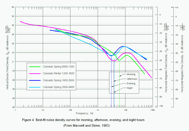
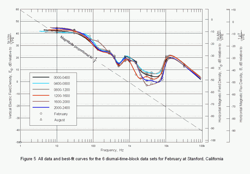
The curves of Figure 4 show less detail than those of Figure 5 simply because the data are averages of time-of-day-block data sets obtained at widely separated (and unspecified) dates, while the Stanford data are from a single month of the year (February) and show considerably more detail.
The curves of Figure 4 show a change in the frequency and magnitude of the "dip" as well as a change in the magnitude of the 10-kHz peak over the course of a 24-hour day. These are probably related to the height of the local ionosphere. The curves of Figure 5, the Stanford February data, show systematic inflections at 150 Hz, 500 Hz, and the peak at 11-12 kHz. The well-defined minima of the Colorado spring data are much broader and generally show decreasing and increasing edges at the same frequencies. (These features do not appear in the way Chrissan and Fraser-Smith portray the data and are not discussed or explained by the authors.) The depth of the broad null shows marked variability over the diurnal cycle, suggesting that either source activity or the local propagation path changes during the cycle (probably both). The 10-kHz peaks in all curves are probably due to the peak of source energy due to the large return-stroke lightning flash energy and also the upper edge of low-VLF attenuation curve seen in figure 6. The very consistent local minimum at 500 Hz is unexplained as is the lesser local minimum at 150 Hz.
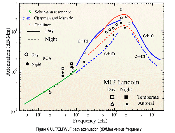
The attenuation graph of Figure 6 is taken from Barr, et al, p 1696, and shows the ULF/ELF/VLF attenuation over the range 5 Hz to 10 kHz due to the earth-ionosphere duct propagation attenuation. Of note is the stability and very low attenuation below 100 Hz, and the variability of the attenuation peak over the two decades between 100 Hz and 10 kHz. This variability seems to be reflected in the Stanford data, but does not explain the 150- and 500-Hz minima. It will be interesting to find out if VLF Open Lab experimenters notice similar irregularities and if they are the same or vary with their locations.
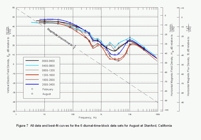
Figure 7 is the graph of a data set identical to that of Figure 5 except it is for half a year later, the month of August. When compared with the February curves, August shows more general variability and higher overall noise density. Between 100 Hz and 12 kHz, the noise level is roughly 10 dB higher. The large minimum between 2 kHz and 8 kHz is less well defined and for the 0800 to 1200 period, almost non existent. The 500-Hz minimum is prominent only during the afternoon hours. The 150-Hz minimum is not apparent at all. These differences remain unexplained. (Data for the remaining months of the year have not been reduced to a form suitable for a magnitude versus frequency lot, but may hold some clues not yet apparent.)
Plots of opposing time-of-day blocks, e.g. 0800-1200 and 2000-2400, have been made for both February and August, but reveal no surprises. These curves are already embedded in Figures 5 and 7 and can be highlighted manually if you print the graphs.
EARTH-IONOSPHERE CAVITY RESONANCE
The resonance phenomenon has been covered in some
depth by Renato, IK1QFK, and will be mentioned here only for completeness.
In 1952, W.O. Schumann predicted the existence of electromagnetic resonances
in the earth-ionosphere quasi-spherical shell cavity. Schumann proposed
that the resonance frequencies are given by,
| fn = 7.49[n(n + 1)]½, for n= 1, 2, 3, ... |
This equation yields f1 = 10.6 Hz, f2 = 18.4 Hz, and so on. It was not until the early 1960s when Balser and Wagner5 of MIT Lincoln Lab, under a contract to study electromagnetic effects of high-altitude nuclear explosions, observed that the nuclear electromagnetic pulse excited the earth-ionosphere cavity and caused resonances. Their measured results of the resonance peaks were somewhat lower in frequency than the proposed Schumann Resonance (SR) frequencies in that f1-5 = 7.8, 14.2, 19.6, 25.0, and 32 Hz. The difference has since been shown to be due to ionospheric losses and not an error in Schumanns proposal. These differences have been used as a diagnostic of propagation conditions.
The SR appear in the 5- to 60-Hz spectra of the output of your receiver as bumps in the noise profile at approximately the same frequencies noted by Balser and Wagner. However, it is (hopefully) lightning that is exciting the cavity and not nuclear detonations. The SR probably appear as spectral "bumps" rather than discrete spectral lines because of the ionospheric propagation losses that cause the downward shift in frequency and also because the excitation is a non-coherent series of impulses rather than a long single-frequency pulse.
Earlier we mentioned that the ionosphere in the presence of the geomagnetic field is a birefringent medium. The splitting of a propagating wave in a magneto-ionic medium into ordinary and extraordinary components is essentially the Zeeman Effect normally associated with optics. The ordinary and extraordinary waves propagate at different velocities and appear at slightly different frequencies. This could account for the peak splitting sometimes seen in the SR.
CONCLUSION
The reviewed data have illustrated that propagation at ELF/VLF frequencies is affected by a large number of interactive variables. The result is a natural noise spectral density that is both consistent and inconsistent, depending on the frequency band of interest. Global path attenuation up to at least 100 Hz is low and consistent, but monotonically increasing. The band of frequencies between several hundred Hz and about 8 to 9 kHz is highly variable (generally within 10-15 dB over any particular diurnal cycle and 25-30 dB over a year) at mid-latitude locations. This variability is caused by a number of influences that dynamically change the propagating medium and hence the observed noise level. The 10-kHz region is characterized by a noise peak that is due to both dramatically reduced attenuation and a broad maximum in the lightning return-stroke spectrum. Above 10 kHz the noise power spectral density tends to fall off at 10 dB per decade of frequency increase well into the LF range. This tells us that the propagation medium is more stable and that the noise sources that dominate lower frequencies are not so dominant in this region.
The experimenter can use any of the mid-latitude data shown in Figures 5 and 7 to obtain a good estimate of the ELF/VLF noise spectral profile at any time of day and, by interpolation, any time of year. February and August, at mid latitudes, demonstrate the extremes of the annual monthly-averaged data. Experimenters at low latitudes can probably expect higher noise because of their proximity to the noise sources. Similarly, experimenters at high latitudes can expect higher or more variable noise levels due to auroral effects and ion bombardment from solar events and interaction with the upper geomagnetic field, the magnetosphere. We did not include any high-latitude data in this article, but may do so at some later date.
The multiple and diverse causes of earth-ionosphere duct variability opens the door to a wide range of experiments that are well within the capabilities of amateurs. A few individual experiments that come to mind include:
1_ E.L. Maxwell and D.L. Stone,
"Natural Noise Fields 1cps to 100kc", IEEE Transactions on Antennas
an Propagation, Volume AP-11, Number 3, pp 339-43, May 1963.
2_ D.A. Chrissan, A.C. Fraser-Smith,
Seasonal
Variations of Globally Measured ELF/VLF Radio Noise, Technical Report
D177-1, Stanford University Dept of Electrical Engineering, STAR Lab, December
1996.
3_ R. Barr, D. Llanwyn Jones,
C.J. Rodger, "ELF and VLF radio waves", Journal of Atmospheric and Solar-Terrestrial
Physics, Volume 62, Issue 18, pp 1689-1718, November 2000.
4_ Kenneth Davies, Chapter
9, Propagation of Low and Very Low Frequency Waves, Ionospheric Radio
Propagation, New York, N.Y., Dover Publications, Inc., 1966.
5_ M. Balser and C.A. Wagner,
"Observations of Earth-ionosphere cavity resonances", Nature, Volume
188, pp 638-41, 1960.
PDF version of this article is available here