Adapted and enached from the article
published on Radio Rivista March 2013 with curtesy
of its director Gabriele Villa, I2VGW
|
This project
has a unique genesis, being born during a
discussion with some friends, fans like me
of communications at optical frequencies.
How often it happens, extremes concept
meet together, so the discussion on the
higher frequencies of the spectrum slipped
on the observation of those little
different from zero.
In particular, the band of frequencies from 5 to 35 Hz is characterized by the presence and evolution of various natural phenomena, including the "Schumann resonances". |
 |
Schumann resonances
They
are a group of energy peaks in the portion of the
spectrum of extremely low frequencies (ELF), effect
of global electromagnetic resonances excited by
lightning discharges.
 |
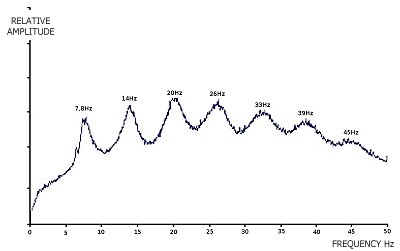 |
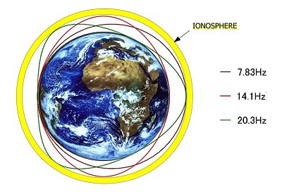
| Figure 1: Example cavity resonance modes | Figure 2: Spectral distribution of the top 5 Schumann resonances |
This phenomenon is named by physicist Winfried Otto Schumann who first predicted it mathematically in 1952.
The
cavity, whose boundaries are the Earth's surface and
the ionosphere, it is naturally excited by energy
from lightning discharges and its resonance is
revealed as separate peaks in the field of ELF
around 8, 14, 20, 26 and 32 Hertz.
Given the nature inherently variable of
the electrical properties and geometry of the
cavity, the "spectrum lines" are actually frequency
bands centered around the frequencies calculated, as
shown in the example herewith shown.
These signals are collected and analyzed for various studies such as example:
- climate studies distribution of lightning
- abnormalities of the ionosphere
- extraterrestrial lightning
- geomagnetic disturbances
- transient luminous events
- seismic precursors
The receipt of these natural signals is usually
carried out by stations specifically equipped, in
which a large antenna or said better, an E field
sensor, is the heart of the receiving system.
But
not everibody is lucky enough to be able to have
room enought to its installation. The aim of this
work, is therefore, to propose some solutions and
practical suggestions to those willing to study the
matter but having limited means. The solution
presented is suitable for field day use, in order to
allow the enthusiast to take advantage of a "day out
of school" for experiment with success.
The system
Wanting
to
simplify at most the schematic of the necessary
elements to this study , we can assume the following
situation: 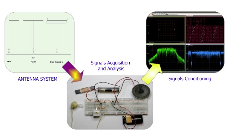
The system is composed of an element designed to capture the natural electric field, followed by a module that processes the signal to make it easy to be analyzed, then the last item, in chargheof the analysis.
Let us now, block by block, develop some considerations of design and use.
The antenna
The newcomers less accustomed to these extremes frequency, could legitimately ask whether it is possible, as in the VLF and higher, use a kind of active antenna, made with a small stylus and an appropriate amplifier stage of high input impedance.
If,
from a theoretical point of view the thought is
logical and motivated, unfortunately some practical
aspects make it very difficult if not impractical
this choice.
Let see with some interesting observations
on this regard:
- an antenna "small", let say a wire of 2 to 3m of length, has an equivalent capacity quite low, about 30 to 40pF. Whether we would linearize its frequency response down to 5 Hz, it must be "closed" (loade with the input resistance the frontend) of about 1 GOhm.
- the "gain" of the small stylus with respect to the electric field to pick up is also very low and this leads to the need to use high amplifications.
The two factors just discussed, leading to having to
design and build a front end very critical, almost
impossible to stabilize outside of a laboratory, and
where few raindrops or a bit of mist may completely
distort the measurements.
It
should worth to be considered how playing with an
antenna very short, every little disturbance of the
static field on its vicinity, becomes a signal or
better, a disturbance in measurement. Flying
insects, the grass moving in the wind, the movement
of some human in the vicinity of the antenna as well
as the atmospheric agents such as rain, fog, snow
are all elements that can create havoc in various
ways on the output signal of the system.
The
Marconi antenna, because of its more generous
dimensions, it solves many of these problems. Also
for the same reasons, it presents a high capacity to
the ground, which allows the design and
implementation of a front end much less critical and
expensive.
The
solution proposed is a compromise between wishes and
real possibilities, with a goal to allow a certain
freedom of study and experimentation.
To
convince definitely the novice about the
difficulties, you can consider how 10 Hz are
associated to a wavelenght of 30.000km. A Marconi
20m long, therefore, it is equivalent to use for the
reception of the medium wave, a whip only 0.2 mm
long!
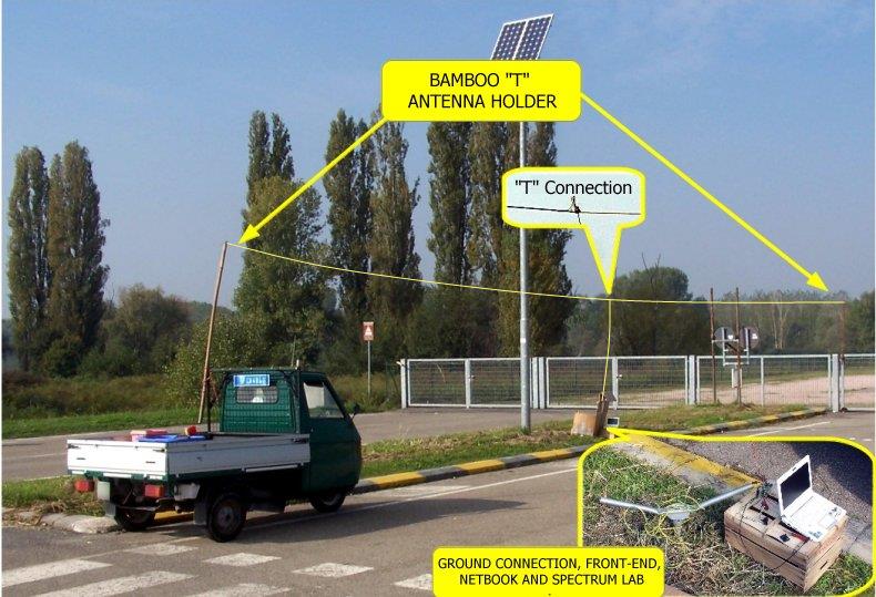
From experiments made with the system described below, it appears that:
- an inverted L antenna, 9m long and 2.5 m high from the ground can be considered an "entry level"
- a T antenna, 18m long and 3m from the ground already allows good "listen" of all resonances
- more bulky structures, of course, allow to appreciate more details of the variability of the signal
The front end
It is the stage that collects the signal received by the antenna and, using an appropriate treatment, makes it available to the device in charge of record and analysis. Its main tasks are:
- Adapt the high impedance of the antenna to the low one of the recorder "manage" the strong signal at 50Hz
- amplify the signal collected at the appropriate levels
- linear response of the system in order to have a sensitivity "fairly flat" in the frequency spectrum of measurement and thus allow quantitative measurements on the signals acquired
- "manage" small overlapping signals with large variations of the input (typical storms for example) without damage
Figure 4: Diagram of the proposed front end
(click here
for full resolution picture)
- R1: defines the input impedance of the circuit and the cut-off frequency of the system "antenna + front end." It also has the task of grounding the bias current of the operational amplifier.
- LN1 is a small neon bulb (without series resistance!), which clamps the input voltage when it rises above 60 ~ 100V limiting in the case of storm, the input voltage to the circuit to a safe level, thus improving its reliability. As much as possible, choose a low-voltage bulb.
- T1 and T2 are two general purpose transistor used as clamp diodes with very low leakage current.
- R2 limits the current in the diodes T1 and T2 in the case of high voltages at the entrance
- L1, R2, C1 realize a low pass filter at about 20kHz to avoid overload from out of band signals
- R15 and R16 determine the gain of the first stage. Depending on the situations it may be convenient to modified it, using the R16 that can then be replaced for example by a potentiometer of 10 kOhm.
The choice of the first integrated circuit
As often happens, the first stage of a receiver is what determines most part of the final result. The choice of the active device is therefore important and must be performed in this case following two guidelines:
- the effect of the bias current of the inputs
- the effect of noise generators
To study the effects of the bias currents of the inputs, we can use the scheme shown here:
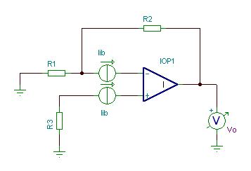
Figure 5: equivalent schematic for the effect of bias current
Considering the values of the resistance of the circuit, it appears that the key role is the difference of potential generated across of R3. Thus, it's important choose a device with low bias current. For the study of the noise we can use the diagram below:
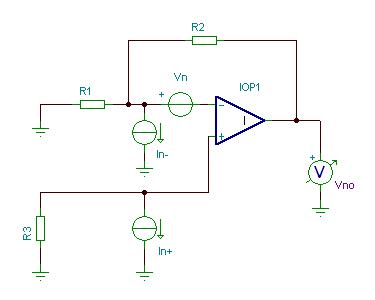
Figure 6: Schematic equivalent for study on noise
The contributions to the total noise are due to:
- thermal resistance
- noise voltage of the operational
- conversion by the resistances in voltage noise of the noise current tof the amplifier inputs
With a little of calculations, we can put in evidence as with the values of resistance employed in the circuit, it is the predominant the contribution of the operational input noise current the to the total noise. By comparison of the performance of some of the devices mostly available, we obtain the following summary table calculated at 10Hz, 17 ° C and with the values of R1, 2,3 of the circuit before described.
Figure 7: Comparative table between different OpAmp
The first six devices are substantially equivalent and considering cost and availability perhaps it may be worth experiencing only the alternative between the TL071 and the AD820. The OP07 and OP27 and following ones, although excellent in general sense, for this specific application are not advised because of their high current noise at those frequencies. The breakdown of the various contributions to the total noise in the circuit, is summarized in the graphics below. Pay attention as the scale is a logarithmic type.
The notch
Even when you operate the system on a remote area, the 50 Hz of the mains network, will be always the louder signal, sometimes strong enought to defeat the acquisition system. Thus, it's introduced a notch filter centered at 50Hz in order to reduce the amplitude of that unwanted signal without affecting significantly the useful band of the system. For its maximum effectiveness should be made of components (Resistors and capacitors) with 1% accuracy.
The second stage has the following tasks
- load properly the notch filter
- introduce a pole in the transfer function of the overall system so to linearize the frequency response
- properly drive the line to the signal analysis system
Final result
Putting "all together" you get the following response of the antenna system and the frontend:
 |
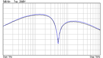 |
| Figure 9: Simulation of the frequency response | Figure 10: Frequency response measured on one of the prototype. In comparison a TL071 and AD820 |
where you can see:
- bandwidth from 5 to 30 Hz within 3dB
- > 30dB attenuation at 50Hz
- roll off above 200Hz to avoid overload by signals well outside the band of interest
The system is powered by a pair of rechargeble batteries of 8.4 V NiMh. With their 140mAh capacity, they are sufficient to guarantee a day of operation of the system. If you need a greater autonomy, you can assume the use of two small batteries Pbgel of 12V or maybe four cells LiPo if the weight factor is important.
The system PC + software
The simplest way today to analyze the signal, is the use of a computer with a sound card and an appropriate software. Unfortunately, not all the sound blaster work fine down to those frequencies and is therefore warmly advisable, to test them before using. As a programs for the acquisition, recording and analysis, among the most popular we can mention:
- Spectrum Lab for capturing and analyzing in real-time
- Baudline & Sonic Visualizer for post processing
Please refer to their websites for each instruction on their use and configuration.
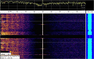
What do I receive?
As anticipated, the system presented offers good reception. In the figure below you can see a recording prepared with Spectrum Lab and acquired with the antenna T of 18m, supported by occasional means as visible in other images.
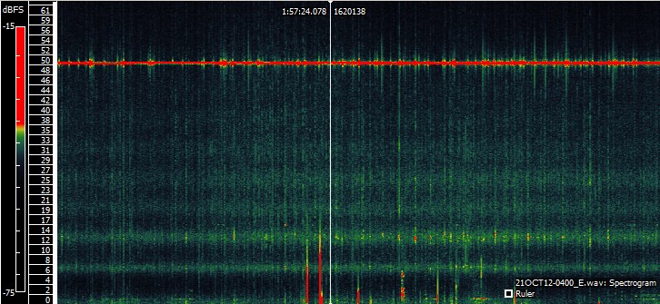
The result is very positive and achieved with little effort and investment.
The bands of Schumann resonances are clearly visible, as well as 50Hz albeit its considerable amount does not affect the cleanliness of the acquisition.
General Guidelines
To drive the testing activities quickly towards an efficient configuration, you can consider the following guidelines:
- where possible, prefer a "T" antenna structure rather than an "L inverted "
- provide means to dampen the mechanical vibrations of the wire as much as possible. For example, the horizontal conductor can be kept in constant traction on one side with a weight that pulls down and dampens the oscillations, thus improving the S/N below 10 Hz
- place the front end to the base of the T and from this point starting with a long shielded cable to carry the audio signal to the PC in the shack.
- place the ground connection at the same point, that is at the base of the vertical section of the T
- it is good practice to put the netbook (or a generic PC) to at least a dozen yards from the antenna and the receiver. This distance is very dependent on the amount of noise generated by the computer and should be checked case by case
- test and experiment with the use of an isolation transformer placed between the receiver and the sound card. It's not always needed, but often it helps.
- another important caution: the microphone input of sound blaster cards almost always deliver some DC voltage to feed a condenser microphone. It should be blocked with a condenser, before it is grounded by the eventual line transformer above mentioned.
- it is better if the electronics of the front end,it is enclosed on shielded case
- each mass that perturbs the static electric field in the vicinity of the antenna is transformed into a signal on the spectrogram, especially below 20 Hz. So, things, or people who move around the receiving system, can create artifacts on the received signal. The establishment of an area "not walkable "around the antenna, at least 10 feet from each part of the receiving structure, can be a good starting point.
- Avoid as much as possible power sources "alternating" for the devices involved. Battery packs are usually the best choice, they do not generate noise and make the whole system "floating".
Ackoledgement
At the end of this paper, I would like to thank Marco and Andrea IZ5IOW, IZ5TLU for having me light up the curiosity on this matter and Renato IK1QFK and Marco IK1ODO for the competent and valuable help and support of experience.
For those
wishing to explore some of the many topics covered in
this article, I may suggest to take a look at the
bibliography.
Bibliography:
Renato Romero, Radionatura, Sandit Libri, 2006 Albino
Pierluigi Poggi, Active antennas, Sandit Libri, 2011 Albino
AA.VV, Low Level Measurements "Keithley
Daniel H.Scheingold, Transducer interfacing handbook "Analog Devices inc. 1980 - Norwood, Massachusetts USA
it.wikipedia.org / wiki / Risonanza_Schumann
http://www.scribd.com/doc/75455378/30/Ilrumorenegliamplificatorioperazionali
http://www.baudline.com
http://www.vlf.it
http://www.glcoherence.org/monitoringsystem/earthrhythms.html
http://www.qsl.net/dl4yhf/spectra1.html