Jean-Marie Polard (F5VLB) – Peter Newton (GM0EZR) – rev 1.1 april 2026
1. Introduction
Very Low Frequency (VLF) signals such as DCF77 (77.5 kHz) and MSF (60 kHz) are valuable probes of ionospheric behavior, particularly within the D-region. Monitoring their amplitude variations provides insight into propagation changes linked to solar illumination and atmospheric dynamics.
Although the UMC series can sample up to 192 kHz, practical measurements above ~40–50 kHz become increasingly unreliable due to anti-alias filtering, amplitude response irregularities and phase distorsion close to the Nyquist limit.
To overcome this limitation, a frequency translation (heterodyne) approach is implemented to shift the VLF signal into the audio band (~1 kHz), where the acquisition system performs optimally.
Note : applicable to both UMC202HD and UMC404HD
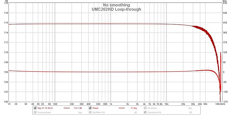
Loop
through spectrum of UMC202HD. Not bad for audio
applications 0… 25kHz.
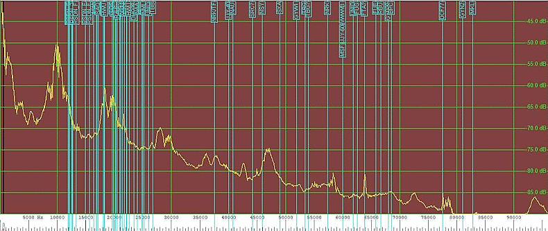
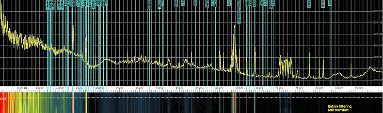
Spectrum
at 192kHz sampling of the band 0-96kHz without
transfert.
 |
 |
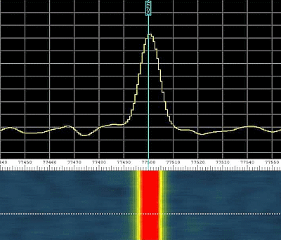
DCF77
native signal and Transfered signal
2. System Overview
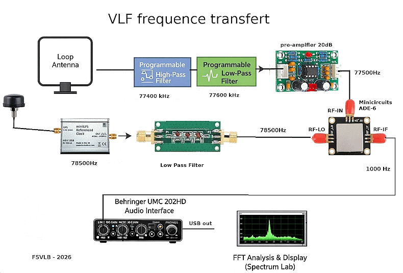
Diagram of
the system
2.1 Signal Chain
- Magnetic loop antenna
- Low-noise VLF preamplifier
- RF band-pass filtering
- Passive RF mixer
- USB audio interface (Behringer UMC404HD)
- Spectrum Lab software (DL4YHF)
The heart of the system
3. Hardware Implementation
3.1 Antenna System
The receiving antenna is a large magnetic loop (~125 m²) installed at approximately 3 meters above ground level, oriented East-West.
This configuration maximizes sensitivity to the magnetic component of the VLF field, provides good rejection of local electric noise, as well suited for reception of European VLF transmitter
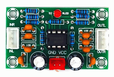
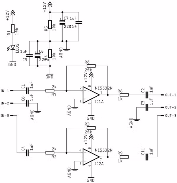
3.2 Preamplifier
| The signal is
amplified using an Audio XH-A902 module, based on
the NE5532 operational amplifier. Although originally designed for audio applications, the NE5532 performs adequately in the VLF range due to the low operating frequencies involved. Low-noise performance, sufficient gain to compensate for mixer conversion loss, stable operation in the VLF range. The idea is to have the same level (gpsdo/vlf signal) at the entries of the ADE-6. |
 |
3.3 RF Filtering
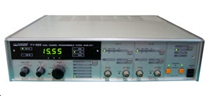
A double programmable filter FV-664 is used as the RF filtering stage. And is implemented as a tunable band-pass filter
- Typical setting (DCF77):
- Lower cutoff: ~77.4 kHz
- Upper cutoff: ~77.6 kHz
Role: Limits out-of-band noise, prevents mixer overload and improves overall signal quality
 |
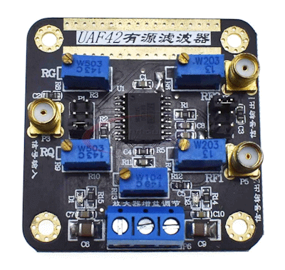 |
The
programmable filter (alternatively you can use a
module UAF42)
3.4 Local Oscillator
The local oscillator is a GPS-disciplined oscillator (GPSDO) from Leo Bodnar.
In the present implementation, the GPSDO output level was adjusted to approximately +7 dBm, compatible with the nominal drive level of the ADE-6 mixer.
Example: DCF77 (77.5
kHz) → LO = 78.5 kHz → output ≈ 1 kHz
This corresponds to a high-side injection configuration: Fout = LO – VLF station frequency
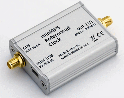
- High absolute accuracy
- Excellent long-term stability
- Reproductible measurement conditions
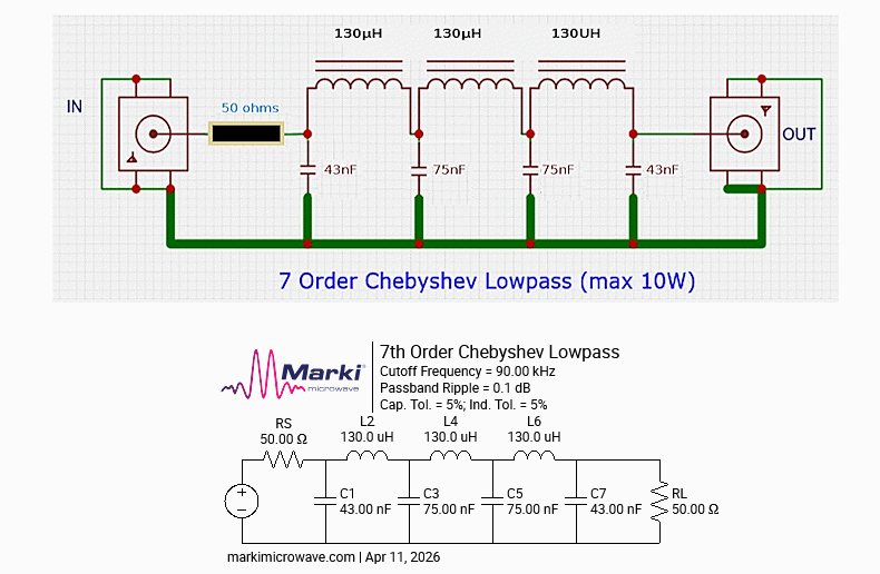
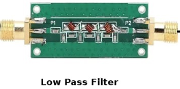
A LPF at the output is required to get sinusoidal wave. (see drawing hereunder).
3.5 Mixer
Frequency conversion is performed using a Mini-Circuits ADE-6 double-balanced passive mixer.
Although the ADE-6 mixer is specified for much higher frequencies, practical tests showed acceptable conversion performance at VLF for amplitude monitoring purposes.
These modules have a wide frequency range, a good port isolation, for a typical LO drive: ~+7 dBm
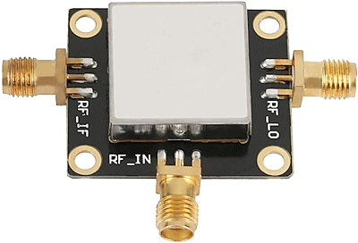 |
RF LO is the entry for 78500Hz RF in is the entry from the double filter RF if is the output to the UMC sound card |
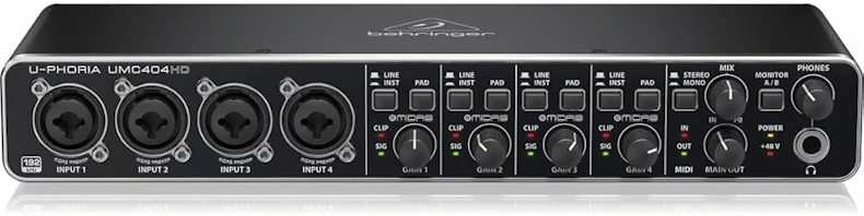
3.6 Acquisition System
The downconverted signal (~1 kHz) is fed into a Behringer UMC404HD audio interface. (an UMC202HD can also be used)
Advantages: Operation in optimal frequency range, flat amplitude response and low noise floor Stable digitization
Use the instrument input (not the line input), no pad, and adjust the volume under clipping,
Input gain must remain fixed during measurements. Any automatic level control, compression, enhancement or software audio processing must be disabled to preserve true relative amplitude variations of the received VLF signal.
3.7 Analysis Software
Signal processing and visualization are performed using Spectrum Lab (DL4YHF). It has a high-resolution FFT, the possibility of ong-term recording, and a narrowband tracking. Spectrum Lab is particularly well suited to narrowband VLF monitoring applications.
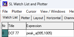
You start with a native Spectrum Lab configuration. You adjust as usual the audio i/o to 192000 and you set the waterfall around 1000Hz where the signal of DCF will be present. Looking around 77500 will show the native signal of DCF (77500Hz) and the 78500 Hz from the gpsdo.
In the watch and plot tag, you have to set the expression as on the picture hereunder.
4. Frequency Translation Principle
The system uses a heterodyne approach:
Fout = LO - Fvlf
With the vlf signal at 77500Hz and LO at 78500Hz the output is 1000Hz. If you want to change for 60kHz tune the system to 59kHz...
5. Filtering Strategy
5.1 RF Domain
• Moderate band-pass filtering (FV-664 or UAF42) and amplification of 20dB to prevents overload and spurious mixing. The RF band-pass filtering is also important to suppress image responses and unwanted mixing products.
5.2 Audio Domain
Optional narrowband filtering around 1 kHz. Improves signal-to-noise ratio.
A conversion frequency near 1 kHz was deliberately selected for several practical and technical reasons. This region is sufficiently far from the mains frequency (50 Hz) and its strongest low-order harmonics, which significantly reduces contamination by power-line interference. In addition, audio ADCs generally exhibit their best amplitude linearity, lowest distortion and most stable response in the mid-audio range rather than near the upper end of their bandwidth.
Another advantage is related to FFT-based signal analysis. Around 1 kHz, standard audio processing software such as Spectrum Lab provides excellent frequency resolution and very stable narrowband measurements with relatively modest FFT sizes. This makes weak amplitude variations and fine spectral structures easier to observe and quantify over long recording periods.
As a result, the translated signal benefits from a cleaner spectral environment and improved measurement stability compared with direct acquisition near 77.5 kHz.
6. Basic Calibration and Validation
The system is designed for amplitude measurements, not absolute phase.
6.1 Frequency Accuracy
- Verified, using GPSDO derived injection and has a stable output at ~1 kHz
6.2 Linearity
Output amplitude proportional to input. No observable compression.
6.3 Bandwidth
Verified over ±100 Hz around carrier
6.4 Noise Floor
System noise vs atmospheric noise distinguished
NOTE – don’t forget to do the calibration of your UMC sound card !
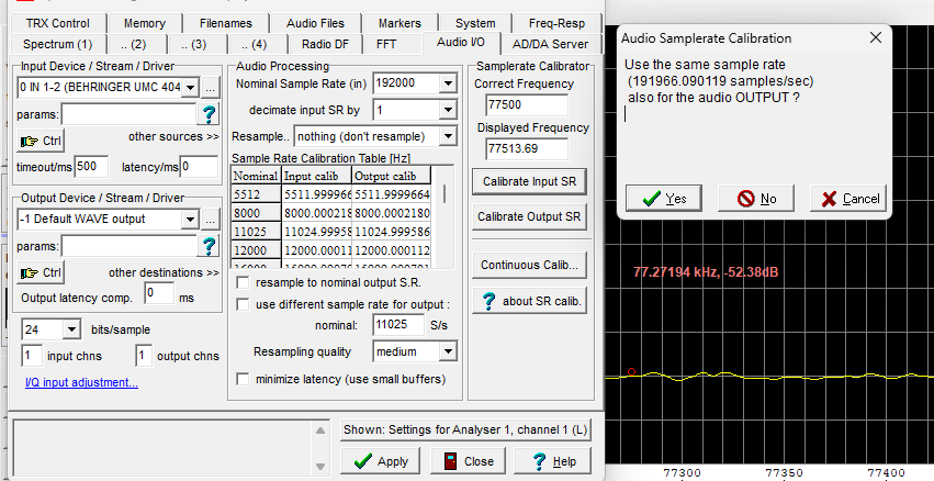
The samplerate calibration procedure should be performed before measurement ! If you stop Spectrum Lab, the audio calibration should be performed !
In the audio i/o tag, enter the correct frequency, the value measured on the screen and click calibrate input SR then YES in the appearing screen. Correct frequency is the one of a known station (i.e. 77,5kHz). With the mouse read the displayed frequency. Click on calibrate SR,and agree the audio samplerate calibration. After some seconds, the system is calibrated.
7. Operational Use
The system enables:
- Stable amplitude monitoring
- Sunrise/sunset detection, SID’s, gravity waves, VLF pollution, meteors reflections
- Day-to-day comparison
- Detection of anomalies
In practice, the region around 1 kHz was found to be significantly quieter than the mains-related spectrum near 50 Hz and its harmonics.
8. Measurement Examples
To illustrate the performance of the system, two types of observations are considered:
8.1 Direct RF Observation (77.5 kHz)
When observing the signal directly near 77.5 kHz the signal amplitude is reduced, the spectral definition is poorer, presence of increased noise and instability are observed
Response depends strongly on the limitations of the audio interface, these limitations make precise and repeatable measurements difficult.
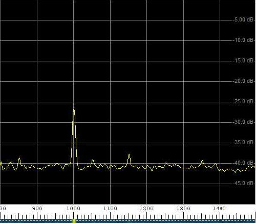
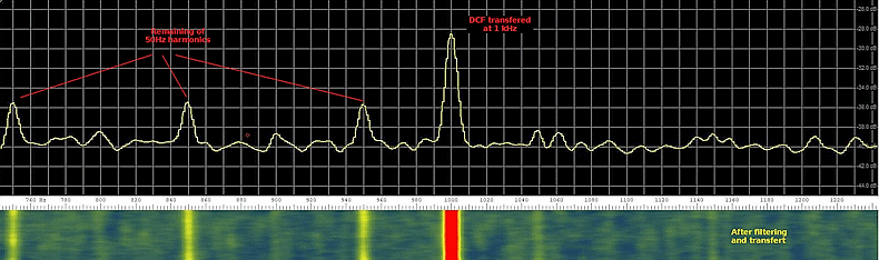
8.2 Downconverted Observation (~1 kHz)
After heterodyne conversion we obtain a clean, narrow spectral line appears near 1 kHz with a signal stability improved and a noise floor ireduced. Now, fine amplitude variations become clearly observable
This demonstrates the benefit of operating within the optimal bandwidth of the acquisition system.
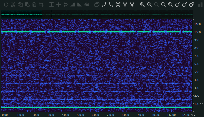
Spectrogram of the converted signal, starting at 0 Hz, generated using OcenAudio 3.13.
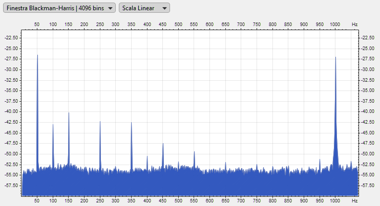
The spectrum, generated using OcenAudio 3.13.
The 50Hz and harmonics are present, but no so strong near 1000Hz. This is why we choosen this frequency for our transfert. Now you can adopt another frequency, the 1000Hz is not mandatory, provided you are in a quiet region of your sound card. Generated using OcenAudio 3.13.
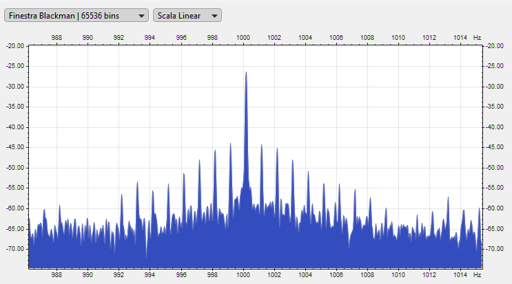
Detailed
spectrum around the signal converted to 1 kHz. Spectral
components related to the 1-second DCF77 modulation
structure are visible around the carrier. Generated using OcenAudio 3.13.
structure are visible around the carrier. Generated using OcenAudio 3.13.
8.3 Visual Comparison
- Spectrum screenshot around 77.5 kHz (direct reception)
- Spectrum screenshot around 1 kHz (after downconversion)
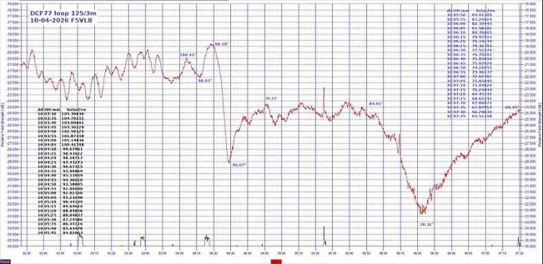
8.4 Observed Phenomena
Typical observations include:
- Gradual amplitude change at sunrise
- Unexplained V drop after sunrise
- Stable daytime plateau
- Nighttime signal enhancement
- Occasional disturbances (sid, ionospheric tides, gravity waves, ...)
These variations are consistent with known VLF propagation behavior in the D-region.
Parameters for the plotter window
You are working now at 1000Hz, not 77500 !
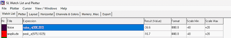
Else the spectrum lab is working as for any measure involving an UMC soudcard. Just look around 1kHz instead of 77,5kHz in the water fall. If you use the watch and plot refer to the parameter hereunder.
9. Uncertainty and Error Budget
Main contributors:
- Mixer: ±1 dB
- Front-end: ±1 dB
- Audio interface (UMC404HD): ±0.5 dB
Combined uncertainty:
Interpretation:
< 1 dB → caution
-
2 dB → significant
The dominant limitation is atmospheric noise rather than instrumentation.
10. Discussion
Strengths : Simple and reproducible, uses accessible hardware, excellent frequency stability, reliable amplitude measurements
Limitations : Conversion loss, requires level control. No phase exploitation at this stage (the measure of the phase with the PAM function is not stable)
11. Conclusion
A GPSDO-based heterodyne system provides an effective solution for VLF signal acquisition using standard audio hardware such as the Behringer UMC404HD.
By shifting signals like DCF77 into the audio band (~1 kHz), the system avoids bandwidth limitations and enables stable, reproducible amplitude monitoring.
This approach forms a solid foundation for ionospheric studies and long-term VLF observations.
The method allows low-cost instrumentation to achieve repeatable monitoring of ionospheric propagation effects using existing VLF time-standard transmitters.
12. Future Work
- Phase measurements were attempted
using the PAM function of Spectrum Lab, but stability
was insufficient for reliable scientific exploitation.
- Multi-frequency reception
- Correlation with solar zenith angle (SZA) and determination of the refraction height.
13. References
- Barr, R., Jones, D. L., & Rodger, C. J. – ELF and VLF Radio Waves
- Wait, J. R. – Electromagnetic Waves in Stratified Media
- Behringer UMC404HD : https://www.thomann.fr/behringer_u_phoria_umc202hd.htm
- Spectrum Lab (DL4YHF) : https://www.qsl.net/dl4yhf/spectra1.html
- Audio XH-A902 module : https://www.amazon.fr/damplificateur-pr%C3%A9amplificateur-XH-A902-op%C3%A9rationnel-puissance/dp/B082VYLXD9
- Double programmable filter FV-664 : extremely rare to find out, search for similar equipment like an UAF42 module
- GPSDO : https://leobodnar.com/shop/index.php?index.php?main_page=index&cPath=107
- Mini-Circuits ADE-6 : https://www.amazon.com/ADE-25-Frequency-Passive-0-05MHz-250MHz-Technology/dp/B07HB198CX
- Low pass filter calculator : https://markimicrowave.com/technical-resources/tools/lc-filter-design-tool/
- Module UAF42 :https://www.amazon.fr/Reland-Sun-universel-passage-filtration/dp/B09QJYQGCB
Return to home page of www.vlf.it