By Ihor Storozh
The idea of the following experiment was to check the practical usage of VLF/LF signals, which can be received with a regular audio interface, for time delay of arrival positioning. It is known that signal propagation time depends on ionosphere and changes with day time, but it is still interesting how much it changes for particular place of reception and what resolution can be achieved. The main focus is on DCF77 station because it is the most known time/frequency reference in the region. Also DCF77, beside common used amplitude modulation, has a phase modulated data to increase time resolution, which is a particular point of interest. Possible usage of few other VLF/LF signals as time/frequency reference was checked as well.
Hardware setup
Hardware setup consists of electric dipole and two ferrite rod antennas from LW/MW receivers. Signals are amplified close to antennas and sent to the microphone inputs of the PC through the FTP cable. PPS output of the GPS receiver is connected to the same audio interface using voltage divider. Total four channels are used: stereo inputs on rear and front panels of the PC. It is possible to use all four channels in synchronous sampling mode with ASIO4ALL driver but then it runs only at 48kHz and introduces a delay of 12 samples between front and rear ADCs. The native audio chipset had SW limitation in its driver, preventing it from running all 4 ADCs at the same time. It also had limited bandwidth of 24kHz. So it was replaced with other one, compatible with high definition audio (HDA) specification. The new one supports 192kHz sampling rate not only for DACs but also for all four ADCs.
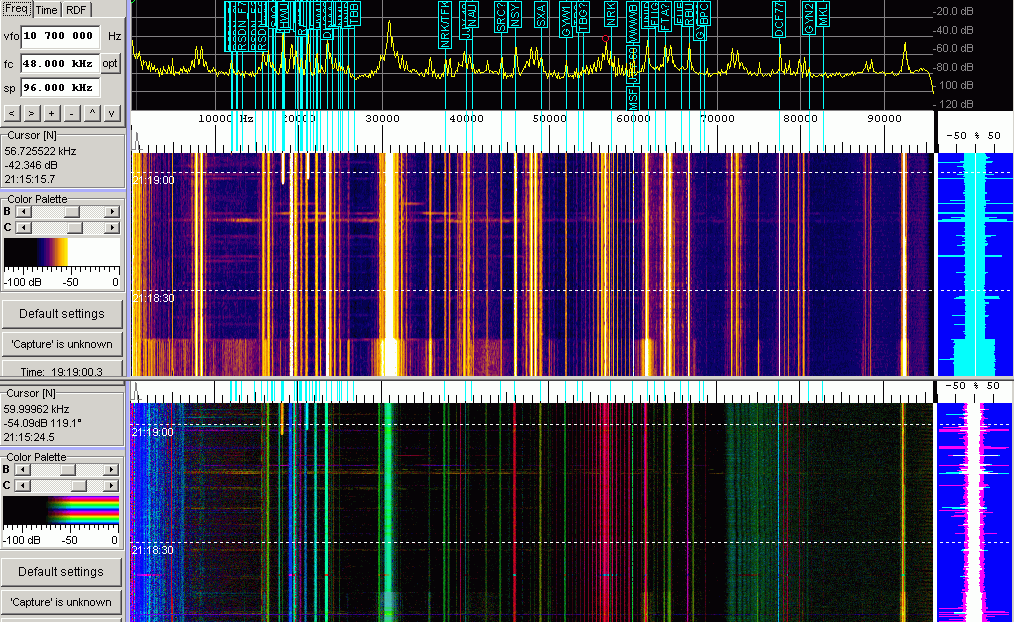
Here is how the signals look in SpectrumLab - electric field at the top and magnetic field from ferrite rodes at the bottom:
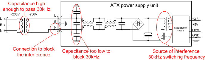
Internal filters of the ATX power supply unit cannot block the 30kHz interference, but since there is already 50Hz 230V to 230V transformer for izolation from mains network, it is possible to connect neutral and earth wires of the ATX PSU together. This effectively bloks the 30kHz and its harmonics.
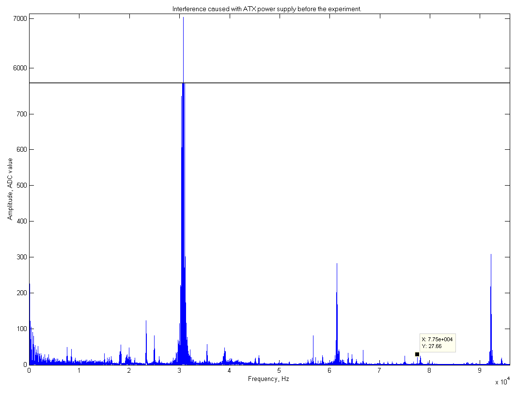
Here is how the spectrum looked in linear scale before proper decoupling and grounding were applied. DCF77 was 252 times lower than 30kHz peak. MSF station was jammed completely. The switching frequency of a power supply unit is not stable, so its harmonics can jam other signals of interest as well.
The electric dipole with differential amplifier was used for reception because it has better signal to noise ratio for DCF77 and MSF.
The software
The goal was to have real-time demodulation and measurement because data stream from ADC is over 6Mbit/s so it can flood the HDD space quickly. All received channels must have the same processing flow. Custom software was writen for the task.
In general the flow should be as following:
- Filtering
- Shifting to baseband (0Hz IF)
- Downsampling
- Demodulation
- Analysis
- Saving calculated data
The first three steps are done with DFT filter. Audio data is buffered in RAM and DFT is calculated using FFTW library. FFTW library allows calculation of DFT from arbitrary data size. 192000 samples was chosen to have a 1Hz/bin resolution. Cosine window with 75% overlapping is used. Then 4000 complex samples of the achieved spectrum, centered at the frequency of interest, are multiplied by filter shape and inverse DFT is calculated. The frequency of interest is a DC bin of the DFT, so spectrum is moved to base band. The output of inverse DFT is a complex IQ signal. Cosine window is applied again to remove spikes at the edges and signal buffers are added with 75% overlapping to restore continuous stream. At the same time it is now downsamped by 192/4=48 times. There is a side effect of such frequency shifting: only shifts which are multiplier of 4 can be used. This is because window is shifted along the signal for 1/4 of its length, causing linear phase shift across the spectrum. For frequency shift for 4, 8, 12, 16 and so on the phase shift is 360 degrees, so no need to play with phase spectrum.
The filter shape for band pass filtering has to be choosen carefuly. Rectangular shape, which looks easy and good at first, produces huge oscillations for signals with amplitude shift keying, so I used cosine shape instead.
GPS PPS signal from Ublox NEO-6M module passes the same flow, to have the same time delay, but it is not shifted in frequency domain.
Amplitude demodulation of DCF77 and MSF are done by simply calculating absolute value of the complex numbers. Bandwidth of the input signal is 40Hz.
However phase demodulation is not that easy. First of all it requires wider bandwidth, which causes it more sensitive to the noise. 680Hz bandwidth was used. During amplitude keying DCF77 signal is 15% of its fill amplitude. This is close to noise level at RX site, so phase is almost random noise. This makes impossible the DC biasing and detrending of the phase samples. The software PLL was implemented to solve this problem by tracking the average phase. PLL time constant for more than one second was selected to minimize error caused by noise. Current PLL phase is used for fine frequency tuning by rotating the IQ samples on its angle. After this, mean angle of complex IQ samples is close to zero and never wraps around 180 degrees. The angle of current IQ sample is the phase demodulator output which reflects only fast changes of informational signal.
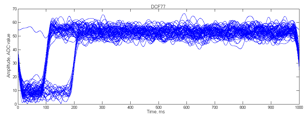
Demodulated phase signal is quite noisy. It is not possible to read the chip sequence from it as is. That is why correlation method must be used here.
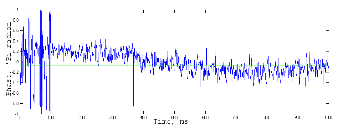
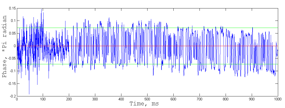
But taking into account the polarity of modulation, which corresponds to the current amplitude keyed data bit, it is possible to accumulate several seconds and see how it looks. Green lines show the +13 and -13 degrees phase span.
So here is the 512bit sequence to correlate with. The C program from Wikipedia can be used to generate the sequence or it can be decoded by accumulating signals during several minutes with precise sampling rate correction.
Now every thing is ready for time delay measurement. But wait, sample rate is only 4000Hz, only 0.25ms resolution is possible if using integer values. Sampled signal does not exceed Nyquist frequency, so information should not be lost.
There is a simple algorithm for finding the peak position of discrete signal by 3 data points using parabolic interpolation. The integer position of the peak must be found first. Its position is considered to be x2=0, previous sample position x1=-1 and next sample position x2=1. The approximated peak position X is calculated from the values of this 3 samples as follows:
d=2*y2-y3-y1; if d is nonzero then X=-(y1-y3)*0.5/d; if d is zero then all 3 samples are equal or x2 is not the peak, so use X=0 to prevent exception.
For finding edge positions of GPS PPS and DCF77/MSF amplitudes the idea from Spectrumlab's sample rate detector is used. The sinc interpolation is used here. The integer position of the threshold crossing is found first. Then a middle point between two samples is interpolated using values of 16 samples around the edge. Its value is compared to threshold and next value is calculated for point moved step towards the threshold. This is repeated for 10 times and step is reduced by half each time, doing successive approximation. This is useful for the GPS PPS, but can be redundant for narrow band DCF77 or MSF amplitude signals if high sample rate is used.
Measurements
The measurements were done for one day. PPS signal was used as a time reference and trigger for writing collected data to the file. The data is stored as 32bit floating point values. The following data is stored:
1. GPS PPS interval between previous and current rising edges;
2. GPS PPS to DCF77 correlation peak delay;
3. GPS PPS to DCF77 amplitude falling edge delay;
4. GPS PPS to MSF amplitude falling edge delay;
5. PLL frequency offset for DCF77, relating to samplerate;
6. DCF77 average amplitude in 680Hz bandwidth
7. DCF77 average amplitude in 40Hz bandwidth
8. MSF average amplitude in 40Hz bandwidth
Let’s first validate the time measurement method by checking GPS PPS intervals. GPS receiver is placed on the window and is connected to the microphone input with long cable. The signal is downsampled to 4000Hz along with RF signals. This is done to simplify the time alignment with other signals, but this also eliminates high frequency interference from mains network.
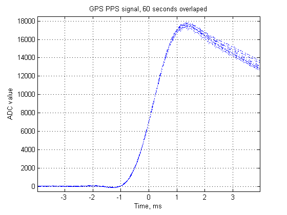
It can be seen that top of the pulse is not flat. This is because of audio codec chip DC blocking feature. Rising edge of the pulse is ok and threshold is set close to the millde of the amplitude.
The interval value between PPS rising edges is saved in seconds as float32. This was actuly bad idea because when value is close to one second the resolution is approx 125ns.
Let's now subtract this one second and see how longer is the PPS period compared to current 4000 samples period.
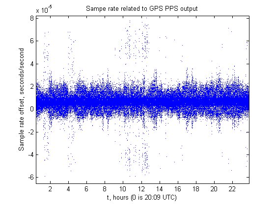
It can be seen that some measurements are out of regular distribution. This is caused with local electro magnetic interference (EMI), affecting PPS signal. However the histogram of the measurements is wery sharp at the top, regardless on the noise:
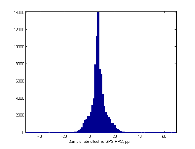
Averaging of such measurements is not good because one big error will significantly affect the mean value. Let's use median instead. This will discard samples with high error. Median is calculated for 60 pulses to have one output per minute. The result is unexpected and exelent. Here it is interpreted as sampling rate frequency offset in parts per milion (ppm):
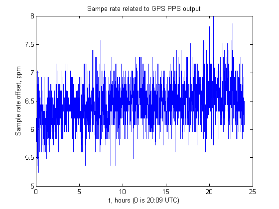
The value of measured sampling rate offset matches the same measured with SpectrumLabs sampling rate detector. Also it shows a very low frequency drift of the audio sample clock over the night.
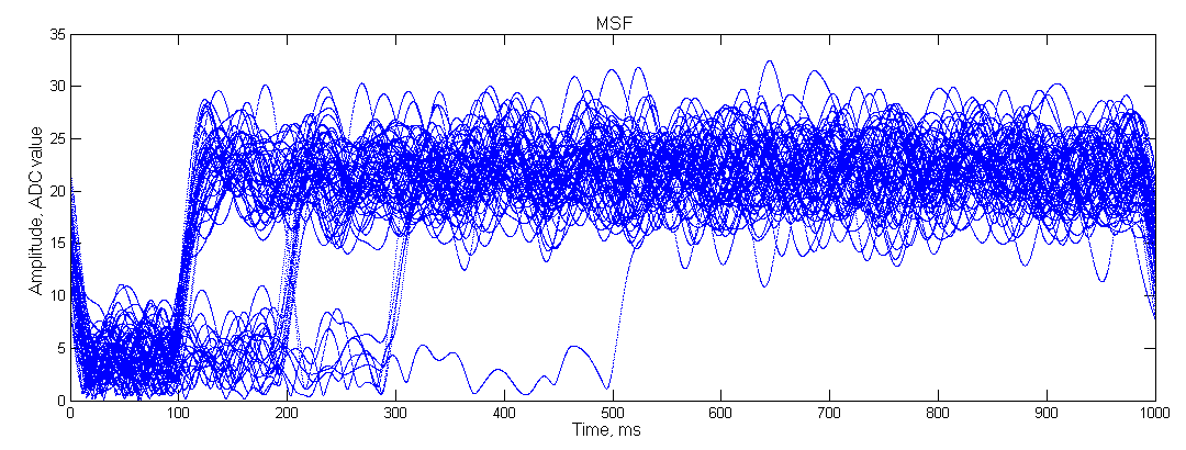
Now let's see the delay of DCF77 and MSF signals taking GPS PPS as a reference. The program counts time delay from PPS rising edge and updates values for DCF77 and MSF when corresponding falling edges are detected. At next PPS the values are saved to file and time counter is reset. Here is a bug because the last detected falling edge is saved even if it was an error or glitch. That is why 200ms is present for MSF. It transmits two bits of data per second, so there is a combination with second falling edge here. Also any noise causes errors which are distributed toward the end of one second.
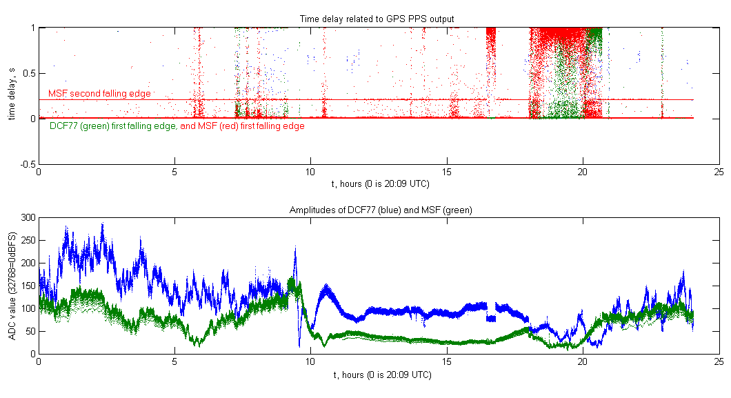
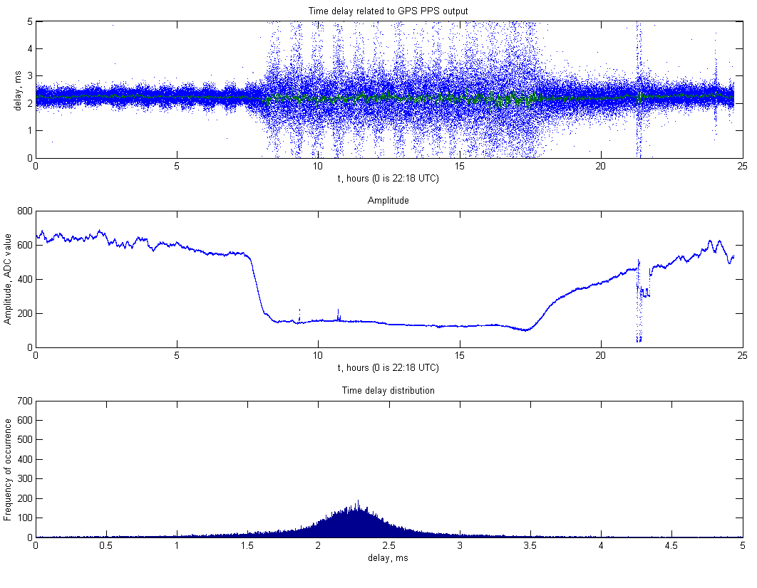
Such a feature of the collected data eliminates possibility of averaging at all. But nonlinear filtering, in particular median, can be applied here as well as for GPS PPS. The same 60 seconds median is applied to amplitude value. It can be seen that errors distribution corelates with low amplitude, but there are also errors with no visible amplitude fading. To have some indicator like signal to noise ratio the ratio between DCF77 amplitudes taken in 40Hz and 680Hz bandwidth is calculated.
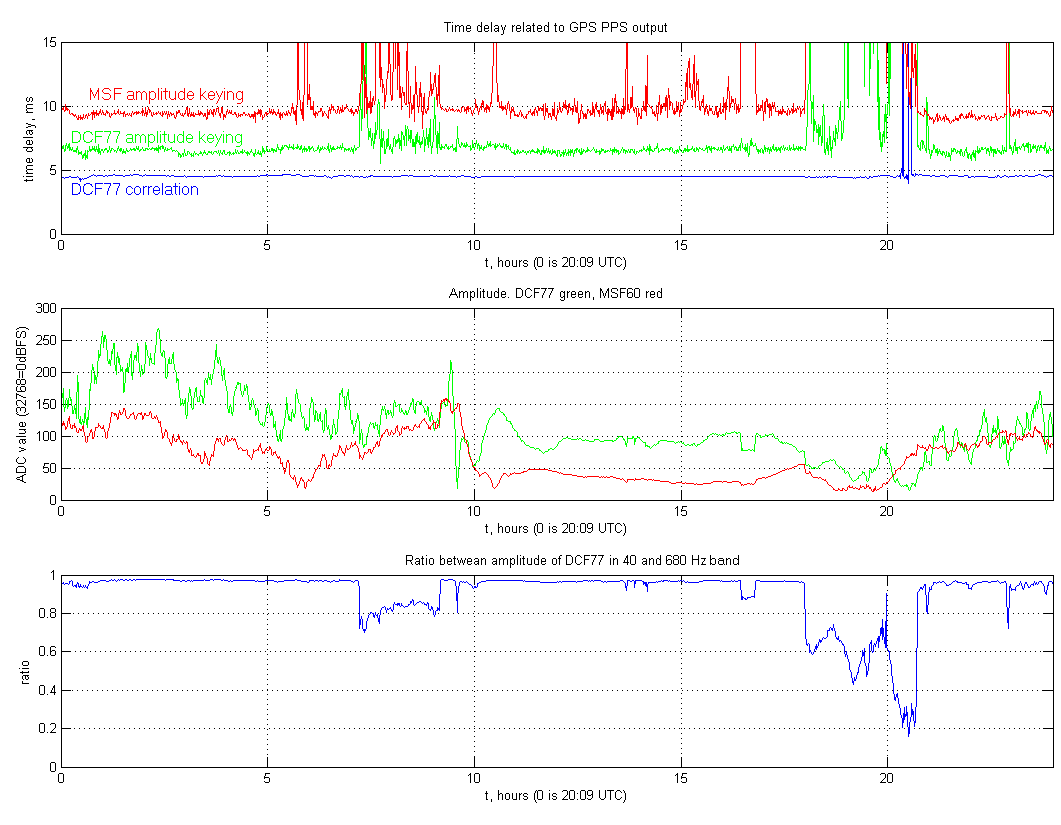
The ratio is close to 1 when DCF77 signal is strongly higher than noise floor and goes down if the inband noise increases. The sadden decrease of the ratio is most likely caused with local EMI which overdriven the input. However the fadeout around 6:00 and 16:00 UTC can be associated with sunrise and sunset events.
The DCF77 correlation is the most stable value all around the clock. The only question here is why the amplitude falling edge is almost 2 ms after it. This can be because the edge detection threshold was set to 58% of the average amplitude, assuming this is a middle point between 15% and 100% of the amplitude (the DCF77 carrier is never turned off completely but keyed to 15% of the nominal level). The threshold for edge detection is adjusted dynamically based on average amplitude. This is like AGC here, but the fact of amplitude keying is not taken into account for average amplitude calculation, so the average value is 80-90% of the real value, depending on data being transmitted. This moves the real threshold to something between 46% and 52%. For MSF the situation is even worse because it has two data bits and a 500ms minute marker.
The distributions of DCF77 and MSF time delay, measured with amplitude keying is shown below. The width of the distributions are several miliseconds. It is clear that these values cannot be used for any kind of position estimation, because 1ms error corresponds to 300km offset on the ground.
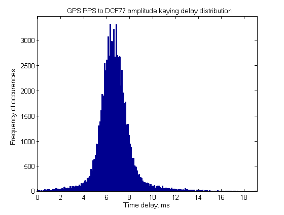
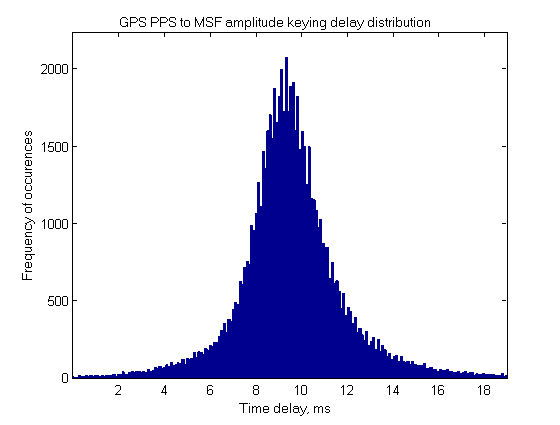
DCF77 is 1075 km away so, in theory, 3.583 ms (surface wave at speed of light) is expected. MSF is 1925 km away with 6.417 ms expected delay. The difference between DCF77 and MSF delays is expected to be dt=2.833ms. The experiment results for amplitude keying are following:
| DCF77 | 6.62 ms |
| MSF | 9.62 ms |
The difference is dt=3.0 ms, only 0.2 ms from expected but the real error is unknown due to edge detection thresholds mismatch.
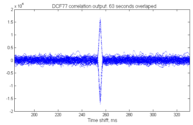
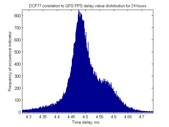
For DCF77 correlation the delay is 4.49 ms which is almost 1 ms more than expected.
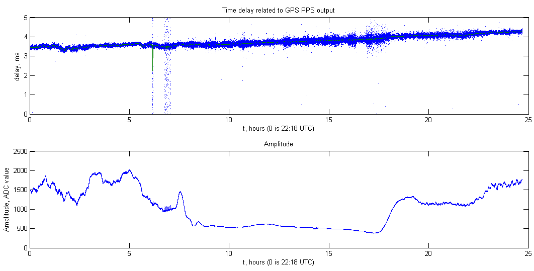
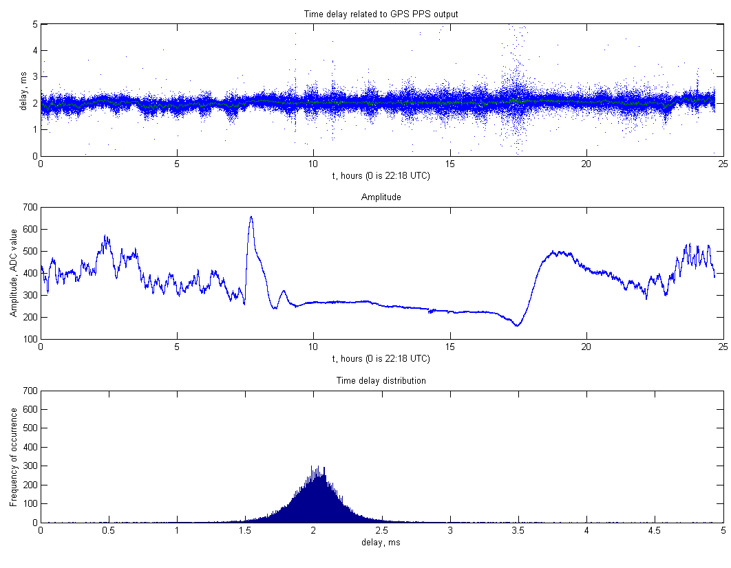
Let's look closer to the time difference of DCF77 correlation and GPS PPS over time.
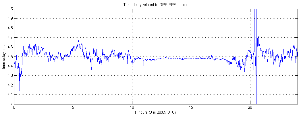
It is stable during day time and changes a lot during night time due to ionosphere conditions. The distribution diagram shows there can be two peaks of most frequent time delay, but is it possible to detect when the sky wave overcomes surface wave and vice versa?
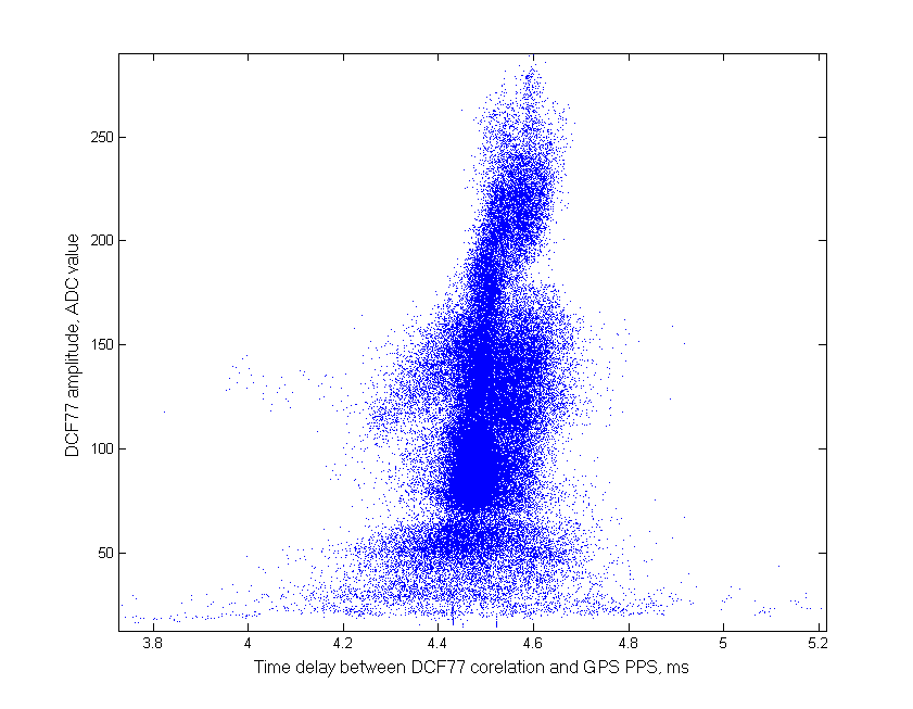
And yes, it can be seen, at higest amplitudes the delay increases. Time difference is only around 100 us and there is no any gap in between, so it seems to be the sky wave all the time, modulated by ionosphere conditions.
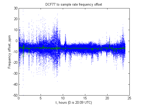
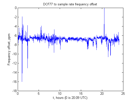
The last part of experiment with DCF77 is to check how stable is the frequency detected with software PLL. Here the detected frequency offset related to sampling rate in ppm is shown. Blue dots are data for each second and green line is median for 60 seconds.
Here is a closer look on 60 seconds median result (1 sample/minute):
Other VLF transmitters
There are lots of other transmissions in the VLF and LF bands. Most of them use Frequency Shift Keying (FSK) or Minimum Shift Keying (MSK) to broadcast data. The carrier frequency cannot be used as a reference because of modulation, but the frequency keying itself may be used as frequency or time reference. The sample rate correction function based on MSK dmodulation is implemented in DL4YHF's Spectrum Lab. The question is how precize and stable the demodulated signals are compared to GPS PPS.
The eye diagram produced by overlapping the demodulated MSK signal for interval of 2 bits is shown below.
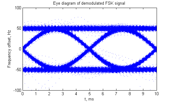
Most of the observed transmitters use 200 bit/s. There are also 100 or 50 bit/s in some cases. This means that zero crossing may appear each 5*N ms. The actual value of N is unknown, therefore a modulo operation with 5 ms divisor is used to eliminate unknown value of N. Time delay is calculated from GPS PPS edge. The 300Hz band pass filter was used for all these signals.
Experiment with MSK signals run over night. Usually the most powerful VLF signal was 23.4kHz but it was not active when the experiment started. There are also strong signals from RDL station (or network) at 18.1kHz and 21.1kHz, but they are active only for short periods so are useless.
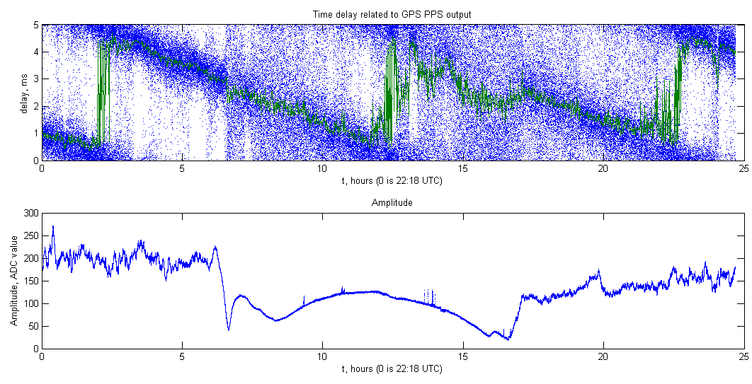
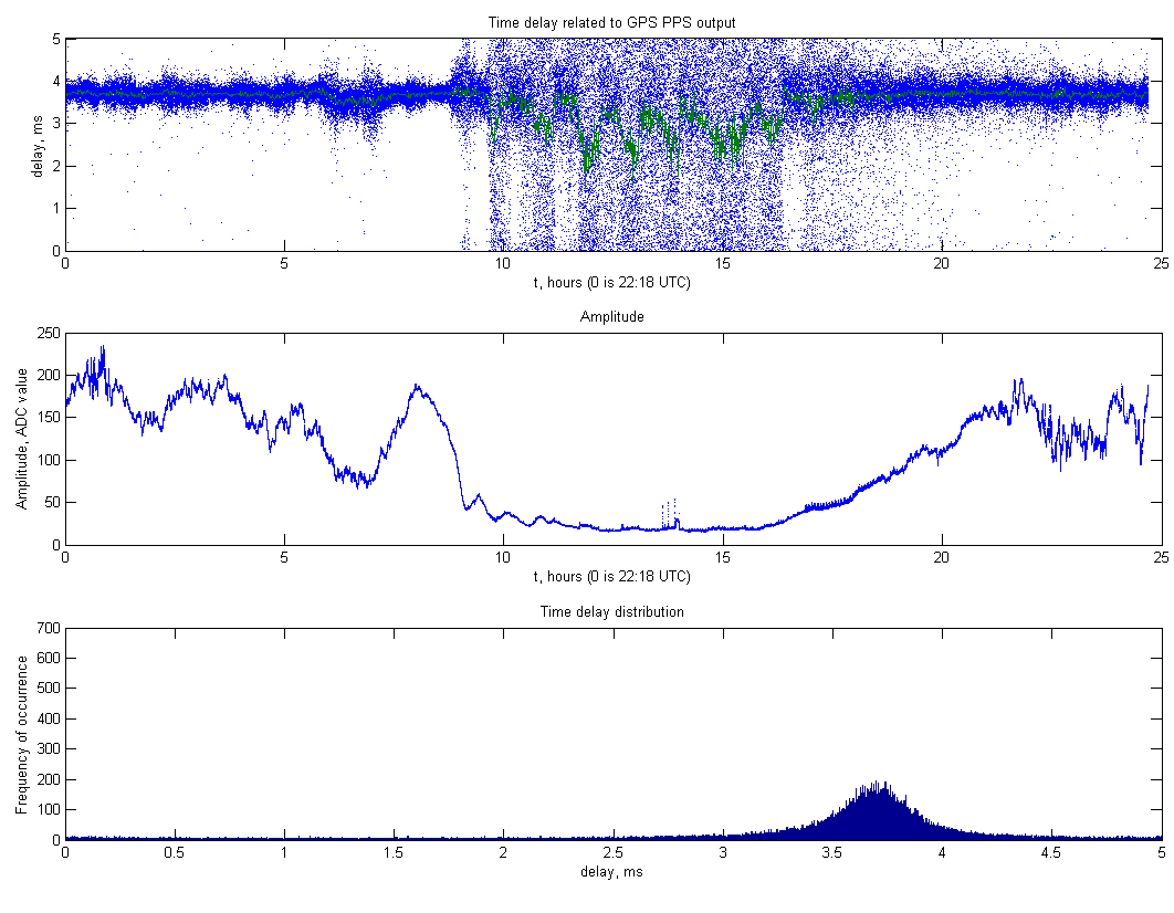
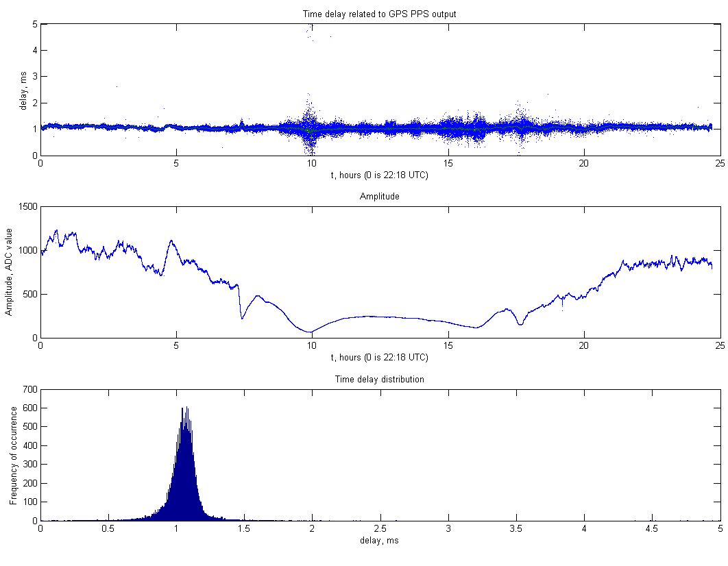
On the below pictures blue dots are data for each second, gren line is median of 60 seconnds.
19100 Hz - unknown source. I checked different VLF stations lists but they all are almost the same and don't mention this frequency. It has not exact baudrate, compared to GPS, but got only 1ms offset over the night which corresponds to 0.01ppm difference (~1s difference for 3 years). So it still can be used for timing applications. The signal is very strong: 10 times of DCF77.
19580 Hz - GQD? G 1922km 298°. The baud rate looks exact and stable. Signal is low at day time and is affected with some interference.
22100 Hz - GQD G 1922km 298°. The baud rate is exact and stable. Signal is stable all the day and only goes low for short time in the evening. This should not be a problem if antenna is tuned to that frequency.
29700 Hz - ? I 1156km 232° or A1F3 ISR 2293km 152°. It is not clear what the actual source is. Signal baud rate is not exact and signal is low.
37500 Hz - TFK/NRK ISL 3130km 317°. The baud rate looks exact and stable. Signal is very low at day time.
45900 Hz - NSY I 1607km 212°. The baudrate is exact and stable. Signal is low only in the morning.
Conclusion
The receptions of DCF77 and MSF time signals is good enough for clock synchronization but signal can be lost for tens of minutes during sunset. Phase modulated signal of DCF77 is almost below noise but can be recovered with correlation method. So this method is even more stable than amplitude method and dropped only for few minutes during sunset. The signal from RBU station was not used due to complicated modulation format (FSK over AM) and also it is affected by local interference.
There are other VLF signals, even below 22kHz, which can be used for time and frequency reference. The time error within 1ms can be achieved with simple filtering. This can be used in places where GPS signal is unavailable or GPS receiver is redundant. Using multiple VLF signals for TDoA navigation with achieved timing precision is useless but there are multiple ways for improvements. Antenna tuned to the frequency of interest may increase the signal to noise ratio. Band pass filter can be optimized for particular station reception. One measurement of MSK edges per second was used in the experiment. Using each edge of the MSK will give up to 100 measurements per second allowing averaging and improving precision.
Return to www.vlf.it home page