By Alessandro VINASSA and Renato ROMERO
It may sound anachronistic, but a device that generates a precision audio time signal can be of great use in a monitoring station for very low-frequency radio signals of natural origin. Let's see why and how to make one with a simple circuit.
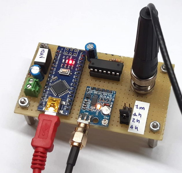
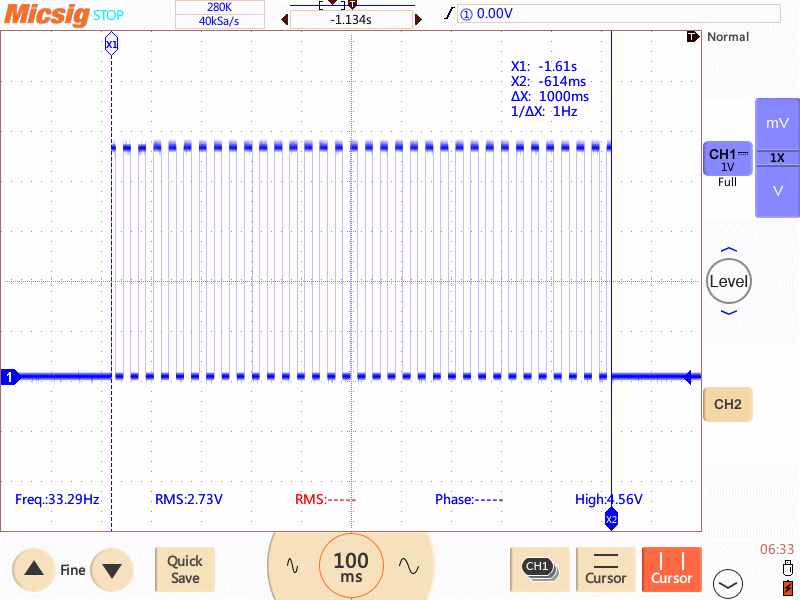
Fig. 1A and 1B The audio marker generator circuit made on breadboard,
and its signal displayed on the oscilloscope: a square wave of 5 V at 33 Hz.
Abstract
What time is it? Each of us asks this question many times during the day, and even more times answers it, saying “it's noon” or “it's 5 PM” or again “it's time to sleep or to eat”. This question seems to be easy because we do not need lots of precision. In everyday life a couple of minutes of error is negligible. Normally mobile’s clocks do not have any indication of the second, limiting their resolution to 1 minute. Considering a computer, the situation is not any happier. Two different PC can show a difference of several seconds in between their clock. You should try to synchronize them using an SNPT server (for example using the program “NetTime”). In this case the error falls to only some tenth of milliseconds because of the various and not completely predictable delay in internet connection. Therefore, it seems we cannot get better accuracy than 10ms.
Indeed, there is another way. The GPS. GPS, or Global Positioning System, serves not only as a precise tool for determining geographical location but also functions as an excellent temporal reference. The accuracy of GPS systems from its reliance on a constellation of satellites orbiting the Earth, each equipped with atomic clocks that maintain incredibly consistent timekeeping. By calculating the time it takes for signals to travel from multiple satellites to a GPS receiver, it can accurately triangulate its position on Earth. This reliance on precise timing is what makes GPS a valuable temporal reference. Flawless synchronization across the satellite network ensures that time is uniformly and accurately distributed, aiding various applications such as financial transactions, telecommunications, scientific research, and even the synchronization of power grids. We are going to use this exceptional temporal precision to generate the absolute time for our vlf monitoring system.
A bit of history, that is: how we were
To understand exactly what a temporal marker generator might have been used for in a VLF signal recording system, it is necessary to take a step back. In the old analog data recording systems, magnetic tape was used for signals, and paper tape was used for plotting. These systems, when compared to a data acquisition card, even something as simple as a sound card, were primitive; today, we would almost call them prehistoric. The limitations were enormous: the magnetic tape system had limited dynamic range, just a little over 40 dB, and the speed of the tape drive motor was unstable, resulting in wow and flutter effects, which also drifted with temperature changes. Additionally, recordings were triggered manually, and the time was noted by hand with uncertainties of a few seconds.
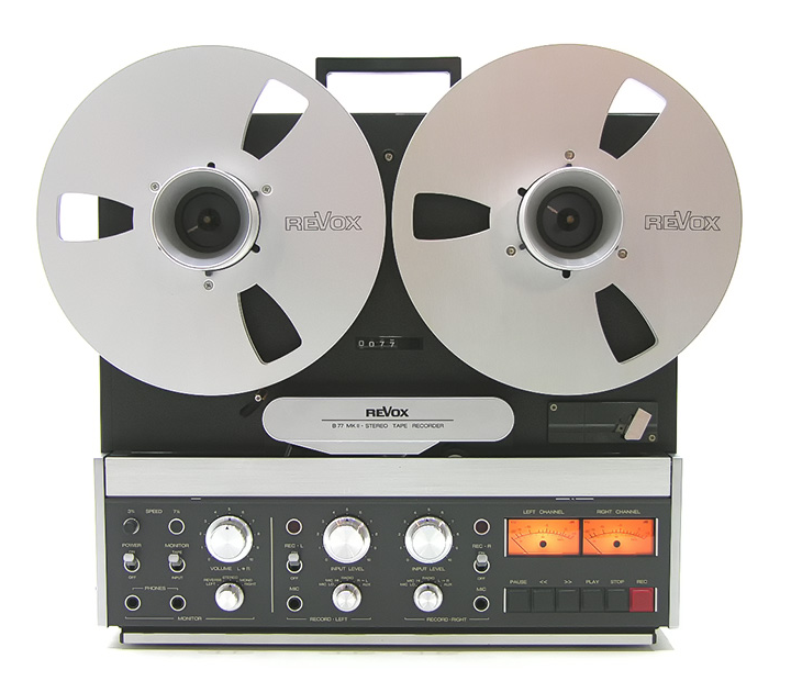
Fig. 2A and 2B. A professional magnetic tape audio recorder, and a chart plotter on tabulated paper.
External devices called "Time Marker Generators" were used to insert precise time references into these records, similar to paper plots. They were an accurate (for those times, that means quartz) clock, which controlled an analog signal generator, for instance, a tone every minute. The time signal was then mixed with the signal from one of the sensors, temporally marking the record. When reading the data, one could then access the recorded data, with the time markers allowing for corrections in reading the recording speed and identifying the exact time of the signals. This way, two recordings made 1000 km apart could be synchronized, enabling them to be compared with each other."
Usefulness of an analog marker today.
But today, with the availability of sound cards featuring 24 bits and sampling rates of up to 96 kHz for Very Low Frequency (VLF) recordings, including time signals like those broadcast on the radio, one might wonder about the relevance of an analog time marker. Does it still serve any purpose? The answer is yes because sound cards do have limitations. It's important to note that these limitations are not inherent flaws of the cards; they are well-suited for their intended general audio applications. But for VLF recordings, a difference on time of 100 ms between two locations can be a problem. Even a slight error on the samplig rate is not noticeable by ear, but on a signal as precise as the ZEVS signal at 82,000 Hz it gives us back the wrong frequency in playback. One or more markers inserted in an audio recording allow us to determine with confidence the time between two points, and thus correct the length of the audio file, i.e., the sampling rate.
But the incorrect sampling rate is not the only problem with recordings made with a PC. Starting recordings automatically, handled by SpectrumLab, also runs into big trouble, even if your PC's clock is being kept synchronized at 10 ms by the SNTP software. When Spectrum Lab sends the "record" command to the PC, it is executed in the queue of other operations that Windows is performing at that time. And we know that Windows always has many things to do! It happens then that a recording commanded for a certain time is triggered on time, but the actual recording starts 400 ms later, for example. This is not a failure of your PC or a malfunction of Windows or Spectrum Lab: it is a limitation of the system.Obviously with professional data loggers this problem does not exist.
These are minor flaws, but if it is necessary to perform a study comparing signals from two or more VLF locations far apart, they become a major problem. Using good quality sound cards, and synchronizing the PC's internal clock with an NTP server unfortunately does not solve the problem. The presence of an analog marker external to the system, i.e., a time signal, is one solution: it allows the duration of the recordings (the samplig rate) to be corrected in a second time and mark the exact time on the recording, allowing them to be almost perfectly aligned to other ones in comparing analisys. Let us see below how it was implemented.
The idea
To understand the behaviour of this project it’s important to have in mind how a GPS practically communicate with the outside word. Many GPS modules communicate with external devices like microcontrollers or computers using the UART (Universal Asynchronous Receiver-Transmitter) protocol. The module sends data as a series of characters through its TX (transmit) pin and receives data on its RX (receive) pin. The transmitted data typically follows the NMEA (National Marine Electronics Association) standard, containing information about position, time, speed, altitude, and more. These data are sent every second. An example of NMEA sentence is the following:
$GPRMC,210230,A,3855.4487,N,09446.0071,W,0.0,076.2,130495,003.8,E*69
Now, it’s not our purpose analyse every field of this sentence, but is important to know that in this sentence, called GPRMC, the first number is the time: in this example the GPS tells us that it’s 9:02PM and 30seconds, UTC time. But when does the 30th second end and the 31st start? That means, when exactly it’s 9:02:30 exactly? To answer this problem, we must introduce the pps signal.
To provide even more precise timing information, some GPS modules feature a PPS output. This is a square wave pulse that occurs exactly once per second, synchronized with the satellite's atomic clock. It does not only have a period of one second, it occurs at the beginning of every second. That means that all the pps signals of all the working GPS are synchronized, having the rising edge exactly at the same time (uncertainties aside, of course). The error in the pps signal, for a commercial, low-level GPS receiver such us the one we will use, is in the order of tens of nanosecond. The PPS signal is used to align the module's internal clock with the global standard time, UTC (Coordinated Universal Time), with extreme accuracy.
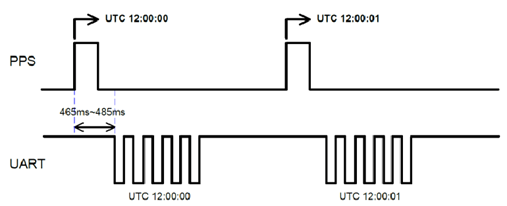
Figure 3: NEMA sentence and pps timing
In Figure 1 it is possible to visualize the relationship between the UART message and the PPS. The UART tells us what the time during the previous rising edge of the pps was. This means that if we receive a time stamp of 12:00:00 UTC from UART, at the next rising edge pps the exact time will be 12:00:01
The circuit
There are several ways to treat a time marker but for this project we have decided to adopt this keyword: Simplicity. But simplicity has drawbacks, and to judge if them can be accepted we must have clear in mind what we want to do.
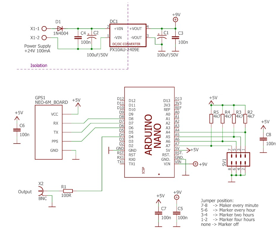
Fig. 4.
The electrical circuit
The idea is to generate an analog marker that can be superimposed directly on the received signal. Our marker will be a square wave of 5V at 33Hz. This signal can be coupled to a small coil placed near the receiving antenna. In this way, the marker will be radiated from our generator to the receiver and can be recorded in a very clear way: no delay, no digital elaboration, no need of dedicated traces. Of course, it can be also be applied to a dedicated channel of the receiver or summed to it. In this last case some care must be taken to avoid noise injection from power supply or from ground-loops. A note about precision. We know that a low-cost GPS receiver can have a timing accuracy in the order of tens of ns. Our marker generator is designed to work with VLF receiver which are normally sampled at 1ksps. If our sampling period is 1ms, is sufficient to have a timing accuracy of less than 0.1ms. Our circuit could degrade the GPS accuracy of 4 orders of magnitude to keep the overall system as simple as possible. And the result is really simple, since a GPS module, an Arduino nano and a few of resistor will do all the job.
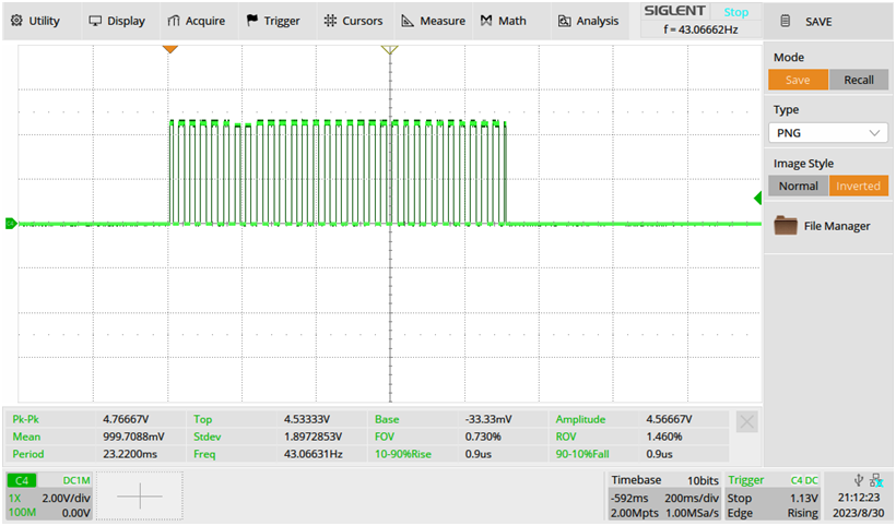
Figure 5: Marker output
A little warning about the gps module. I bought it a couple of years ago. It is a chinese module coming from Amazon. My code works with this module, but I cannot exclude that it may have problems with similar modules (even if from the same series) purchased recently. In fact, I have seen other NEO 6M series GPS modules with different default baud rates or different PPS configurations. Modifications may be required for other GPS. This project is quite experimental. If many readers are interested in it, in the future we could also create a complete PCB.
The heart of the generator is the firmware of Arduino nano. The communication between the Arduino and the GPS is done using the library “TinyGPSPlus.h” in conjunction with “SoftwareSerial.h” that can be both downloaded from the “library manager” of Arduino ide. These libraries are quite heavy, but it has greatly speeded up the development of the project, that was done, as if on its own, in my limited free time. Therefore, oh firmwarists, do not criticize the lack of homogeneity of the program. The firmware of the version we made can be downloaded from here: amg_arduino.zip. If you make a better and working one, I'll gladly throw mine away!
The firmware spends its time reading data from the GPS, which is received through the UART using the "smartDelay(900)" function. Each time a data packet is received, the UTC time indication is automatically extracted from it. A function named "checkTime()" determines whether it is necessary to activate the marker in the next second. If activation is required, the variable "Gate" is set; otherwise, it is cleared.
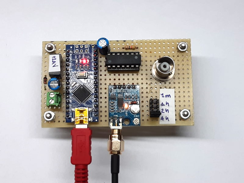
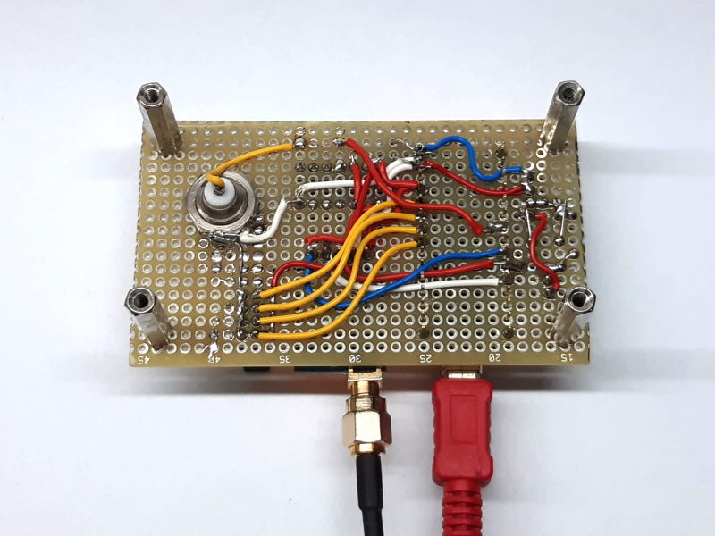
Fig. 6A and 6B. The realization on breadboard, component side and connection side, made with wire.
Subsequently, the program begins monitoring the PPS (Pulse Per Second) input. When the GPS drives this input high, the firmware activates the 33Hz output if the "Gate" is set. Conversely, if the "Gate" is cleared, the firmware stops the 33Hz output. At this juncture, the firmware re-enters the "smartDelay(900)" function, where it awaits for 900ms while reading the UART. By the conclusion of this duration, the GPS message is received, and a brief summary of the time and positional parameters is transmitted through USB. Following this, the "checkTime()" function is once again invoked, and the entire program recommences within an endless loop. What is the compromise? Well, there exists a specific and unpredictable delay between the moment when the GPS establishes the PPS signal and the moment when the Arduino detects this change and generates the corresponding marker signal. In the worst case the tis delay is 24µs, but its average value of this delay, as you can see form Figure 2. The upper trace is the pps, while the lower trace is the marker output. I have superimposed 100 markers.
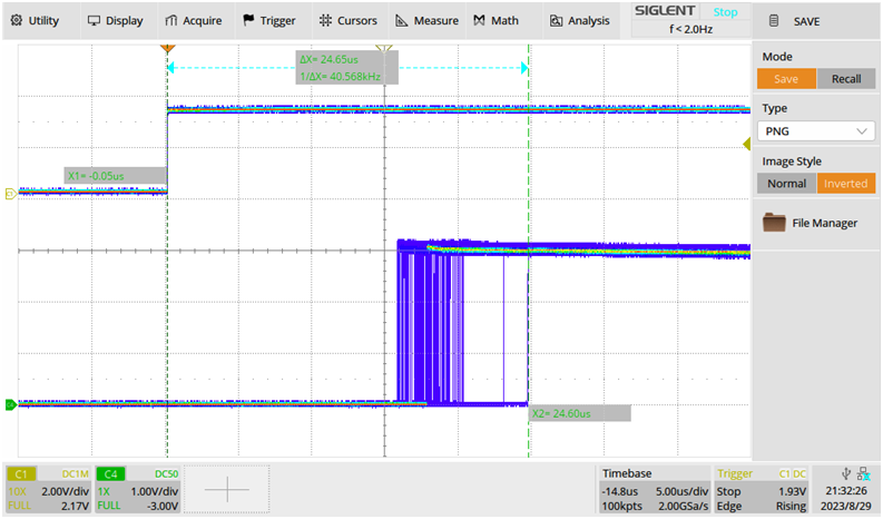
Figure 7: propagation time between pps (upper trace) and marker output (lower trace).
The output of the marker is a square wave directly generated by the microcontroller. To limit the current output I place a 50Ω resistor. The maximum DC power that Arduino can source is 40mA, so keep attention not to short the output for a long time.
This circuit can be powered either directly with the Arduino usb at 5V or from 24V connector. I have placed an isolated DC-DC converter to transform a 24V input supply into 9V. This converter also provides galvanic isolation. This voltage is then regulated to 5V with the on-board Arduino LDO. Using the 24V connection the noise produced from the computer is minimized but you can’tmonitor the GPS status from the USB. We will speak more on this later. The frequency period of the marker can be selected with a jumper. According to the jumper position it’s possible to generate a marker every minute, every hour, every 2 hours, and every 4 hours. The counting of the hours starts from midnight. If no jumper is placed the generator is stopped. After changing the position of the jumper, the generator waits 4 seconds before changing the configuration.This can be very helpful during the process of connecting the marker generator to the receiver (as discussed in the last chapter). To verify the connection, it is beneficial to set the marker every minute to fine-tune either the injection resistor or the antenna's position. After successfully testing this connection, the marker can then be programmed to operate at the desired timing interval.
GPS status monitor
Connecting the Arduino’s USB to the PC have a log of the satellite data via Serial port. It’s possible to use the Serial monitor of the Arduino ide or any other serial interface. The communication parameters are the following: 115200Baud, 8 bits packet, 1 stop bit, no parity. In Figure 3 a screenshot of the serial data:
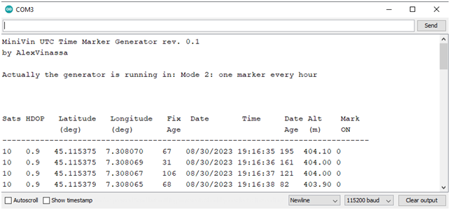
Figure 8: screenshot of the Arduino communication of GPS status
It could be useful a short description of this parameters:
• SATS: this is the number of the connected satellites.
• HDOP: stands for Horizontal Dilution of Precision. It's a parameter used in Global Positioning System (GPS) and other satellite navigation systems to provide an indication of the accuracy and reliability of the horizontal position (latitude and longitude) calculated by the GPS receiver.
HDOP is a dimensionless number typically ranging from 1 to 10 or more. The lower the HDOP value, the better the accuracy of the GPS position fix. A high HDOP value indicates a poor geometric distribution of satellites in the sky. This can be due to factors like tall buildings, mountains, or dense foliage obstructing the view of satellites, which can lead to lower accuracy in position calculations.
Opposite, a low HDOP value suggests a better geometric arrangement of satellites in relation to your position. When the satellites are well spread out across the sky and not concentrated in a single direction, the accuracy of the position fix is generally higher. In practical terms, a common guideline is that an HDOP value below 2 is considered good for most navigation purposes, while values between 2 and 5 are acceptable. Values above 5 can start to degrade the accuracy of the position fix.
• Latitude and longitude: These parameters are self-explanatory.
• The term "fix age" in GPS refers to the amount of time expressed in milliseconds that has passed since the GPS receiver calculated its most recent position fix. In other words, it indicates how old the GPS position information is. This parameter is particularly relevant in scenarios where real-time or up-to-date positioning information is important.
• Date and time: UTC date and time.
• Date Age: it refers to the amount of time expressed in milliseconds that has passed since the GPS receiver last received a valid date and time signal from the satellites. Date age is particularly important in applications that require precise and accurate time information, such as financial transactions, network synchronization, and timestamping. In scenarios where the date age is much more than a second, the time reported by the GPS receiver might be outdated or incorrect. This can potentially affect the accuracy of actions that rely on accurate timing. In summary, the date age parameter in GPS helps users understand how recently the GPS receiver's clock was synchronized with the GPS system time. A lower date age indicates more accurate and up-to-date time information, while a higher date age suggests that the reported time might be less reliable due to the passage of time since the last synchronization.
• Alt: altitude above sea level.
• Mark ON: this variable is set to one if a marker was generated at that time.
Practical application
Once the gps antenna is connected and the system is powered, it is necessary to wait some minutes to keep the gps to track the requires satellites. It is better to place the antenna directly over the sky, without any physical obstacle. Its location can be checked monitoring the parameter HDOP, which must be less than 2 for the best results. Note that the USB transmission in triggered from the PPS: no satellites, no PPS, no PPS no USB monitoring info. The configuration message, however, is printed at every power on. Once the gps is starts to work, its led starts to blink and, therefore, the Arduino TX led stars to blink very smoothly once a second.
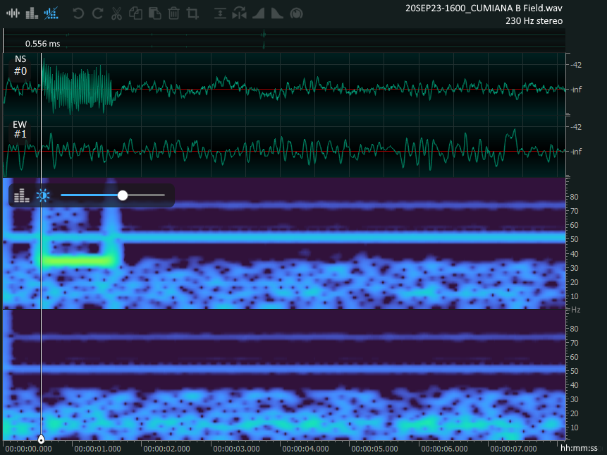
Fig. 9.
First seconds of beginning of a 4-hour stereo recording,
signal from two induction coils placed in the NS and EW
directions.
The start of the was programmed at 00:00:00, and the time marker of 33 Hz was injected directly on the L-channel line (NS coil).
Spectrogram made with Ocenaudio software.
The start of the was programmed at 00:00:00, and the time marker of 33 Hz was injected directly on the L-channel line (NS coil).
Spectrogram made with Ocenaudio software.
And here is an example of a wave recording, made automatically with the Spectrum Lab program, on the signal from two induction coils. The sampling rate is 230 samples/sec. On the recording was placed our 33 Hz marker, on the Left channel of the sound card, in this case corresponding to the coil receiving signals in the North-South direction. The recording was scheduled to start at exactly 00:00:00 (at midnight) but our time marker reveals that in fact the PC, despite being synchronized with an NTP server, started the recording 556 ms earlier.
How to inject the marker signal into our system
An important warning: the marker generator circuit must be placed away from the sensors. This is because Arduino, like all microporocessors, during its operation radiates audio-band signals. This signal would be captured by the sensors fouling the reception.
But let's move on to the marker: the time signal generated by our device is an electrical signal. It can be inserted into the signal reception chain in three different ways. Let's look at them together.
1) DIRECT INJECTION: The signal output from the device can be injected into a signal line, simply by inserting a high-value resistor in series. By signal line we mean the section of cable connecting the VLF receiver to the LINE input of the sound card. With a resistor with a value of 470 kOhm we get an effective signal on the line of a few milliVolts. This becomes, on a spectrogram produced with SpectrumLab, a level of about -45 dB, that is, in the middle of the sound card's dynamic range. This is a good compromise: the time marker is clearly visible, without dirtying the spectrogram too much.
If the incoming signal from the receivers is high and a more robust marker signal is needed, the value of the resistor can be decreased: using a 47 kOhm resistor, for example, the marker signal will have an increase of 20 dB, compared to using it with the 470 kOhm resistor. The method injects the signal on the line, so it is valid for both types of receivers: electric field signals (Marconi and stylus antennas) and magnetic field signals (aerial loop and induction coil). With this method, the marker signal is injected onto the signal line, just as an audio mixer would, mixing it with a signal already there.
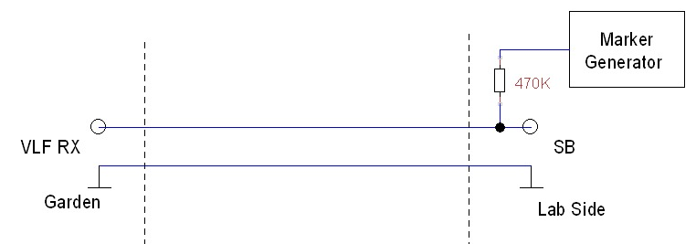
Fig.10. Direct signal injection to the audio line.
2) INDUCTION OF A FIELD: An alternative to direct injection on the signal line is the generation of a field, so that it is received directly by the sensors. The advantage is that the signal line between the receiver and the sound card is not touched. The disadvantage is that the signal from the marker generator must be carried by an independent cable to the sensors, where a device will be placed to radiate it. Let us see how to proceed to induce an electric field and to induce a magnetic field.
a - ELECTRIC FIELD: The circuit generates the signal, and a shielded RG58-type cable, or a twisted pair, carries it to the point of use. At the point of use, near the electric field receiver, a resistor terminates the signal by acting as a load. The hot pole goes to a transmission stylus, the cold pole goes to ground. The weak field generated with this system is sufficient to mark the signal at the input of an electric field receiver, which uses a vertical stylus or large wire antenna as an antenna. To get more signal bring the transmitting stylus closer to the receiving antenna. To get less signal move it away. A 1-meter-long transmitting stylus placed 2 m away from a large Marconi antenna generates a signal at 33 Hz that is 25 dB higher than the natural background noise.
Fig.11. Induction of an electric field.
b - MAGNETIC FIELD: A passive multiturn aerial loop, e.g., forty square loops of side 50 cm, when passed through by current, induces magnetic field detectable even 10 of meters away. At 33 Hz, the impedance of a loop of this size can be very low; therefore, it is necessary to insert a resistor in series with the loop. With a 100 Ohm resistor in series, placing the transmitting loop 8 meters away from the receiving loop or coil, our marker will have an intensity of about 190 pT, which is more than 50 dB above the natural background noise at 33 Hz.
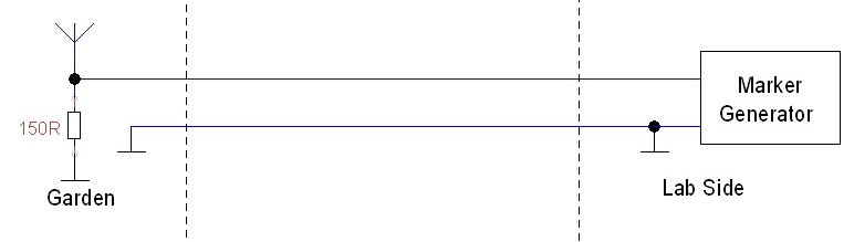
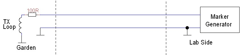
Fig.12.
Induction of a magnetic field.
Conclusions
A simple circuit, a very small expense, and a few hours of work with a soldering iron. But a very useful device, generating an accurate time marker, to give our audio recordings a safe time reference. An indispensable item, if the recordings are to have scientific validity, and are to be used in conjunction with other recordings, for the study of radio signals of natural origin.
Return to www.vlf.it home page