Minivin

MiniVin ACQBoard: From Hobbyist Project
to High-Precision Signal Acquisition
By Alessandro VINASSA

In this article, we present the design of what appears to be a high-performance sound card. It is actually a true data logger with professional performance: a low-cost device for ELF band signals, to be used with SpectrumLab, synchronized with GPS and DC coupled.

Introduction

Let’s start with the problem: monitoring ultra-low frequency signals in the ELF band. These signals can come from all sorts of sources—a geophone, an induction coil, grounding rods, even a Marconi antenna. They might represent magnetic fields, electric fields, or sound waves. In practice, we’re talking about things like Schumann resonances, geomagnetic pulsations, local earthquakes, or distant seismic events (teleseisms). In professional labs, the devices used to capture these signals are called samplers, ADCs, or loggers. Audio interfaces, on the other hand, are a sort of compromise: cheap, easy to handle, but technically limited. Let’s break it down.

Audio interfaces:

Affordable—usually under €200.
No programming required; free software like SpectrumLab lets you monitor in real time and record without being a coding wizard.
Save recordings in WAV format, which can be analyzed with free tools like Audacity, Sonic, or Ocenaudio.

However:

High-pass cutoff of a few Hz means some signals never make it through.
Background noise is fairly high, reducing sensitivity at the lowest frequencies.
Sampling rates can drift, making advanced analyses—like phase correlation between multiple stations—tricky, if not impossible.

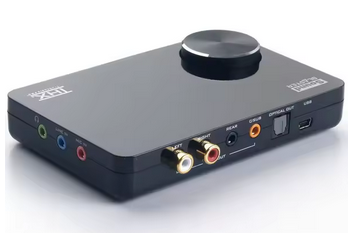
Fig. 1 - A powerful sound card, the Creative X-FI: an excellent compromise between price and quality.

Professional loggers:

Expensive, usually over €2000.
Often require some computer know-how to produce spectrograms and manage data archives.
Save in formats like MiniSEED or proprietary types, which can’t be read by standard audio software—hello, Matlab.

But they shine where it matters:

DC-coupled, so no low-frequency cutoff.
Very low noise at low frequencies, making them highly sensitive.
Usually GPS-synced, so sampling is rock-solid, perfect for advanced analyses and comparisons across stations.

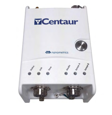
Fig. 2 - A professional multi-channel data logger from Nanometrics,
available in various configurations and price ranges, which also records to SD cards.

So, audio interfaces give you ease-of-use and affordability, but with technical compromises. Professional loggers give you top-notch performance, but at a steep price and with extra headaches.

Now, imagine if we could get professional logger performance from a humble audio interface. That would give us an affordable device, capable of serious monitoring, yet still manageable with free software and zero programming. Enter the MiniVin. This two-channel sampler delivers professional-grade performance, yet can be handled via Wolfgang Buscher’s SpectrumLab almost like it’s just another audio interface—no rocket science required.

Alright, with all of that in mind, let’s jump into the article! I hope this has piqued your curiosity and made you eager to read on. Let’s get started!

“We’ve Always Done It Like This” – Comic introduction

Historically, as you may already know if you've poked around this site before, VLF acquisition has relied heavily on sound cards. They’re cheap, available, and reasonably capable. You sample the audio, run some FFTs, look at beautiful spectrograms, and feel like you’re one with the ionosphere. But—there’s always a but—sound cards come with baggage. Nasty baggage. Renato and I stumbled across this while deep in one of our traditional, highly rigorous technical brainstorming sessions

SCENE: An Italian summer afternoon. Mosquitoes humming. Laptops open. Heat shimmering.

Me: “Red lorry, yellow lorry, red lorry, yellow lorry…”
Renato: “What?”
Me: “Nothing. Vocal warm-up. It helps the brain process FFT bins.”
Renato: “…You’ve had three beers.”
Me: “Fine. Four. But it's here, in this exact state of mild dehydration and complete relaxation, that true innovation is born.”
Renato: “Speaking of innovation, look at this: my software now saves a VLF recording every 4 hours automatically.”

Me: “Nice! Wait… why are these files different sizes?”
Renato: “Ah. The clock drifts.”
Me: “…the what drifts?”
Renato: “The sound card’s clock. So the sampling frequency is not exactly 44kHz. It’s more like 43,999kHz. Or 44,001. You get the idea.”
Me: “But the system is programmed to stop the recording every 4 hour.”
Renato: “Yeah, but the audio card says otherwise. If the card is slightly fast or slow, after 4 hours you’ll get a few seconds more—or less—of audio than you expect.”
Me: “So we can't even measure the timing of an event precisely?”
Renato: “Not unless you enjoy being ± hundreds of milliseconds off.”

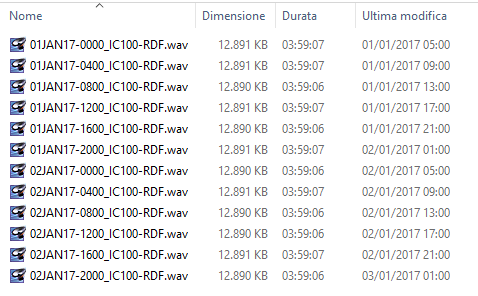
Fig. 3 - Four-hour files automatically recorded with SpectrumLab and captured with a sound card. The duration is similar but not identical, as is the file size. The total duration is also incorrect: each file appears to be missing almost a minute. In reality, it is the sampling rate that is incorrect.

The Sampling Frequency Is a Lie Your Sound Card Tells You

At first, this felt like a funny anecdote—until we realized it’s a serious limitation. You can sync your computer to an NTP server like time.google.com or pool.ntp.org, sure. You can even get really high precision under ideal conditions.

But here’s the catch: NTP syncs over Ethernet and Ethernet has delay. That delay is variable, depending on network load, router buffering, phase of the moon, and possibly beer consumption. Even in good conditions, you're easily off by 10 to 100 milliseconds, and that’s if you’re lucky and your NIC isn’t busy fighting with your RGB keyboard for PCIe bandwidth. And let’s be real: your sound card isn’t listening to NTP anyway. It’s just sampling away at its own leisurely pace, unaware of the absolute time.

In short:

You don’t know exactly when something was recorded.
You don’t know how long a recording truly is.
The PC saving date and time is more of a suggestion than a fact.

But even if you somehow nailed the start time perfectly, there’s still a deeper issue: sampling frequency is not exact, and it is not stable. Your sound card’s clock is driven by a crystal oscillator. Crystals drift. Temperature changes, aging, supply noise: they all contribute. The result is a slow, continuous error that quietly accumulates. This becomes a serious problem when you try to compare recordings from multiple devices, align long recordingsor erform low-frequency or long-term analysis. To understand why, we need to quantify this drift. Suppose we sample at 1 kHz, and consider a frequency stability of about 50 parts per million (ppm). Over a period of 4 hours, how many samples could we be off by?

4 hours = 4 × 60 × 60 = 14,400 seconds

At 1,000 samples per second the total number of samples in 4 hours are 14,400,000

With 50 ppm stability, the drift in samples is:

14,400,000 × 50 × 10^-6 = 720 samples

That means after 4 hours, the timing could be off by as much as ±720 samples — more than a second at 1 kHz! This drift is quite significant and cannot be ignored, especially when you want to compare simultaneous recordings from multiple devices. Without proper synchronization, even small timing errors accumulate, making it difficult to align or analyze data accurately across different units. Solving this problem is trickier. It means telling our device exactly where it is in time continuously, not just syncing the start time.

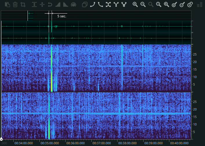
Fig. 4 - A classic example of a signal detected with two induction coils in two locations with a sound card, where the events do not correspond in terms of time, even though both PCs are synchronized with a time server. The time difference between the two recordings is approximately 5 seconds..

Then came the second revelation.

“Why Is There Nothing (or almost) Below 5 Hz?”

When looking at the spectrograms, something odd immediately stands out. In the lower frequency range—the most interesting and information-rich region for VLF—there is almost nothing. Not cosmic silence, but a far more disappointing kind: instrument-induced silence. The reason is a combination of two well-known but often overlooked limitations of consumer sound cards. First, most sound cards are AC-coupled. The input signal passes through coupling capacitors that block DC and very low frequencies, effectively creating a high-pass filter. This alone already attenuates signals as frequency decreases. Second, there is flicker noise, the infamous 1/f noise. Unlike white noise, flicker noise increases as frequency goes down, precisely where we would like the system to be quiet. When these two effects interact, the outcome is particularly brutal for low-frequency work. As frequency drops, the gain rolls off due to AC coupling, while the noise floor rises due to flicker noise. Below a few hertz—often below 5 Hz, and in many sound cards even below 20 Hz—the usable signal is effectively wiped out. In short: the gain decreases, the noise increases and the spectrum turns into a wasteland.

For VLF applications, this is not a minor inconvenience: it is a fundamental limitation of the measurement chain itself. So there you have it. Three foundational reasons why we felt the need to move beyond sound cards:

Timing is unreliable, and events can’t be timestamped accurately to better than ~100 ms (if you’re lucky).
Sampling frequency drifts over time, so even the duration of a recording is uncertain and long-term alignment between devices quickly breaks down.
Low-frequency performance is poor, thanks to flicker noise and AC coupling, which effectively erase useful information below a few hertz. We had started with two problems.

At this point, the list of limitations is already long enough — and if we keep going, it will start multiplying like rabbits. So before things get completely out of hand, it’s time to stop listing problems and start fixing a few of them.

The First to Fall: Flicker Noise and DC Coupling

Luckily, this particular problem turned out to be relatively easy to address: choose the right analog-to-digital converter. After a careful—if slightly obsessive—selection process, we settled on a device from Texas Instruments: the ADS131M02. The name sounds more like a safe combination than a component, but in reality it is a two-channel, simultaneously sampling ADC. In other words, exactly what we needed. Let’s unpack why. The ADS131M02 contains two fully independent ADC cores. This is not a multiplexed input, nor a time-shared sample-and-hold stage. Each channel has its own converter, and both channels sample at exactly the same instant. This detail matters. Many so-called “stereo” ADCs sample one channel slightly before or after the other, introducing a small but measurable time skew. Here, synchronization is enforced in hardware. The result is true simultaneity between channels, which is essential when timing relationships carry information—such as in phase measurements or source localization with microphones. Each channel is naturally differential, although in our case we operate the device in single-ended mode. More importantly, the inputs are DC-coupled and do not require negative supply rails. Thanks to an internal low-noise charge pump, the input can swing from –2 V to +2 V while the entire system runs from a single 3.3 V supply. No tricks, just solid analog design. This capability is crucial. It allows us to record very slow signals, including DC and near-DC components, without running into the low-frequency cutoff imposed by AC coupling. Signals from geophones, electromagnetic field sensors, or ultra-low-frequency biological sources can be acquired directly, without bias injection, coupling capacitors, or the familiar low-frequency roll-off that quietly erases everything below a few hertz. Amplitude stability is equally important. The internal reference is bandgap-based, with a temperature coefficient of just 20 ppm/°C (max) over the –40 °C to +125 °C range. In practice, this means that gain remains stable across a wide range of environmental conditions—whether in a lab, outdoors, or somewhere considerably less comfortable. Each channel also includes its own programmable gain amplifier (PGA), with selectable gains from 1 to 128, allowing low-level signals to be amplified before conversion. And finally, the part that really matters for low-frequency work: noise. The ADS131M02 is a sigma-delta ADC, and its PGAs are chopper-stabilized amplifiers. Both techniques exploit noise shaping to push unwanted noise out of the band of interest. The result is a very low noise floor where it actually counts—at low frequencies—making the device particularly well suited for applications that conventional sound-card-based solutions struggle to handle.

So, what is noise shaping?

Imagine starting with a problem you can’t simply eliminate: ADC’s conversion noise. Broadband, unpleasant, unavoidable noise. If you can’t get rid of it, the next best thing is to move it somewhere else. That is the core idea behind noise shaping.

Noise shaping does not reduce the total amount of noise; instead, it redistributes it in frequency. The goal is to push quantization noise away from the low-frequency band—where the signal of interest lives—and move it toward higher frequencies, where it can be effectively filtered out. This is exactly what happens in a sigma-delta ADC. The input signal is oversampled at a very high rate, often tens or hundreds of times higher than the final output sample rate. A feedback loop then converts this high-rate bitstream into a high-resolution digital output. In the process, quantization noise is no longer flat and evenly spread across the spectrum. Instead, it is shaped: its power is concentrated outside the band of interest. From a mathematical perspective, it is as if the noise were passed through a high-pass filter.

A similar strategy is applied in the analog front end, at the amplifier level. The programmable gain amplifiers in this device use chopper stabilization. At low frequencies, amplifier noise is dominated by flicker noise, also known as 1/f noise. Chopper stabilization tackles this by modulating the input signal up to a higher frequency region, where flicker noise is much lower. The signal is then amplified and demodulated back to baseband. The result is an amplifier whose low-frequency performance is largely immune to flicker noise. For applications that involve signals below a few hertz—or even near DC—this makes a dramatic difference. Where traditional op-amps would slowly bury the signal under drifting offsets and low-frequency noise, a chopper-stabilized front end preserves the information cleanly and predictably.

Clock and Stability Superpowers

Now, let’s move to the Last big issue: you see, even though we have synchronized the time markers perfectly, there is still the notorious random walk of the ADC’s oscillator — the audio card’s clock drifting slowly over time. The issue of sampling frequency stability, as we’ve seen, is quite a complex challenge to solve. However, this analog-to-digital converter provides us with excellent tools to tackle it. In fact, as mentioned, the reference clock is external and must be provided by the user—by us, in other words. This clock, at 8.192 megahertz, needs to be fed into a dedicated pin on the device. So, what’s the approach? Since this device operates by division and uses that reference clock, the stability of the sampled data will depend on how stable that external clock is. Therefore, we decided to go straight to the source, so to speak, and choose the most stable option available for generating that external clock. Initially, we considered a rubidium oscillator, but rubidium is expensive, complex, bulky, and power-hungry. So, we moved forward and thought about a GPSDO. GPSDO technology is well established and has been around for a long time, so why not use a GPSDO? Of course, it will be a simplified GPSDO: it isn’t professional-grade timing-metrological device. It hasn’t all the high-end phase noise and spectral purity that might be required for other applications. There won’t be an expensive oven-controlled oscillator here; instead, we’ll use a much simpler commercial VCXO (voltage-controlled crystal oscillator) to produce the frequency for our microcontroller. This VCXO will be voltage-controlled and adjustable.

Then, we’ll have a GPS receiver that generates a PPS (pulse-per-second) signal. This PPS is sent to the microcontroller, which measures the time difference between its internal timer—running at one kilohertz—and the nearest rising edge of the PPS. This way, we can determine whether the microcontroller’s frequency is drifting higher or lower, and we can correct it accordingly. The correction is done through a 32-bit PWM digital-to-analog converter, filtered by a third-order Sallen-Key filter, and the controller itself is essentially proportional. Why? Because the integral aspect is already embedded in the phase measurement, which, as we know, is the integral of the frequency. This simplifies the controller considerably.

So, what’s the benefit here? The benefit is that with this system, using just a simple external antenna, we can achieve an extremely precise and stable sampling frequency in real-time, without needing any complex synchronization with a computer or external servers. And not only that, we can also know the exact time and date, and this information will be used for the markers, which we’ll describe later. The idea behind these markers is simple: for example, we might have a signal giving us a marker every 4 hours from 00:00:00 UTC time, read from gps. With that absolute time reference, we can pinpoint events and manage low-level timing simply by counting the samples, since the sampling frequency is rock-solid and defined by the GPS and its PLL.

And what if the GPS antenna is not present? Well, without the antenna, there are no satellites in view. This means the precise timing signal (the time markers generator) and the PPS synchronization reference are lost. In such cases, the board signals the error through LEDs on the panel. However, it continues to operate without issues, keeping in mind that the sampling frequency remains stable but with the same stability characteristics as a typical commercial audio card. Additionally, the time markers and related messages will be disabled, since the system won’t receive the NMEA strings necessary to know the exact time. In other words, the system is fully usable both with and without GPS.

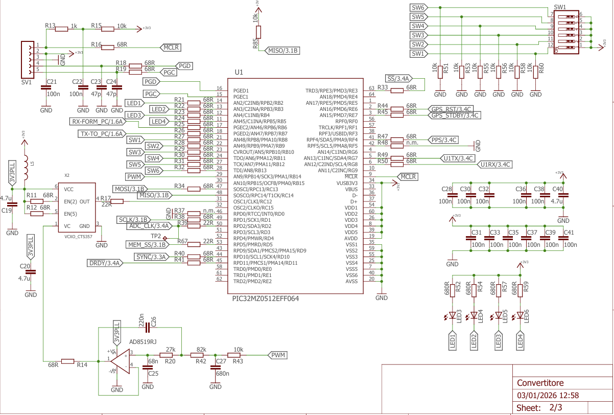
Fig. 5 - Microcontroller section, with all components for GPSDO

At this point it could be useful to understand how the board works in the first place: how the data is handled, what options are available, and what makes this little piece of hardware interesting.

The board gets its raw data from the ADC via SPI. For the sake of our sanity (and a more relaxed debugging session with Renato), we decided to set the board’s sampling rate to a nice, round 1 kHz. This makes the most of our chosen ADC, which has an impressively low noise floor at such frequencies.

Now, here’s the twist: the ADC itself actually runs at 8 kHz. Why? To make life easier for the anti-aliasing filter. In this case, we went for a simple RC filter—because, given the modest 4 kHz input bandwidth and the fact that we’re using a sigma-delta ADC running in an oversampled mode, we simply didn’t need anything more exotic.

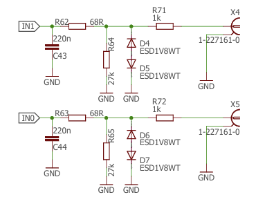
Fig. 6 - The analog input stage: note the simple anti-aliasing filter and the ESD protection

The digitized data then flows into a PIC32MZ microcontroller. Working with this chip is a bit of a double-edged sword: you get fine, low-level control of everything (which is vital for this project), but it also requires a good stock of patience—and occasionally, some colorful language—during configuration.

From there, the data is collected into “pages” at 8 kHz, then passed through a brick-wall FIR filter with a passband of about 350 Hz. This stage performs the first downsampling, bringing the rate to 1 kHz. Once at 1 kHz, the fun begins. The board can be reconfigured in software to sample at 500 Hz or even 250 Hz, each time using an excellent IIR anti-aliasing filter with more than 80 dB of stopband attenuation—meaning no unwanted aliasing makes it through. You can see the frequency response of the antialiasing filters in the figures below

At 1 kHz only, you can also engage a digital notch filter at either 50 Hz or 60 Hz to completely remove the mains fundamental. This can be handy for data visualization, and in some cases also during recording.

Gain is software-selectable from ×1 to ×32. A digital high-pass filter is also available to remove DC drift from slow signals. However, keep in mind that this is a purely digital filter: if the ADC input saturates, the filter won’t save you—it will just see a flat-lined signal.

These processing options were deliberately kept simple but effective. Combined with the ADC’s low flicker noise and solid dynamic range, they provide a flexible yet robust foundation for a variety of low-frequency measurement applications.

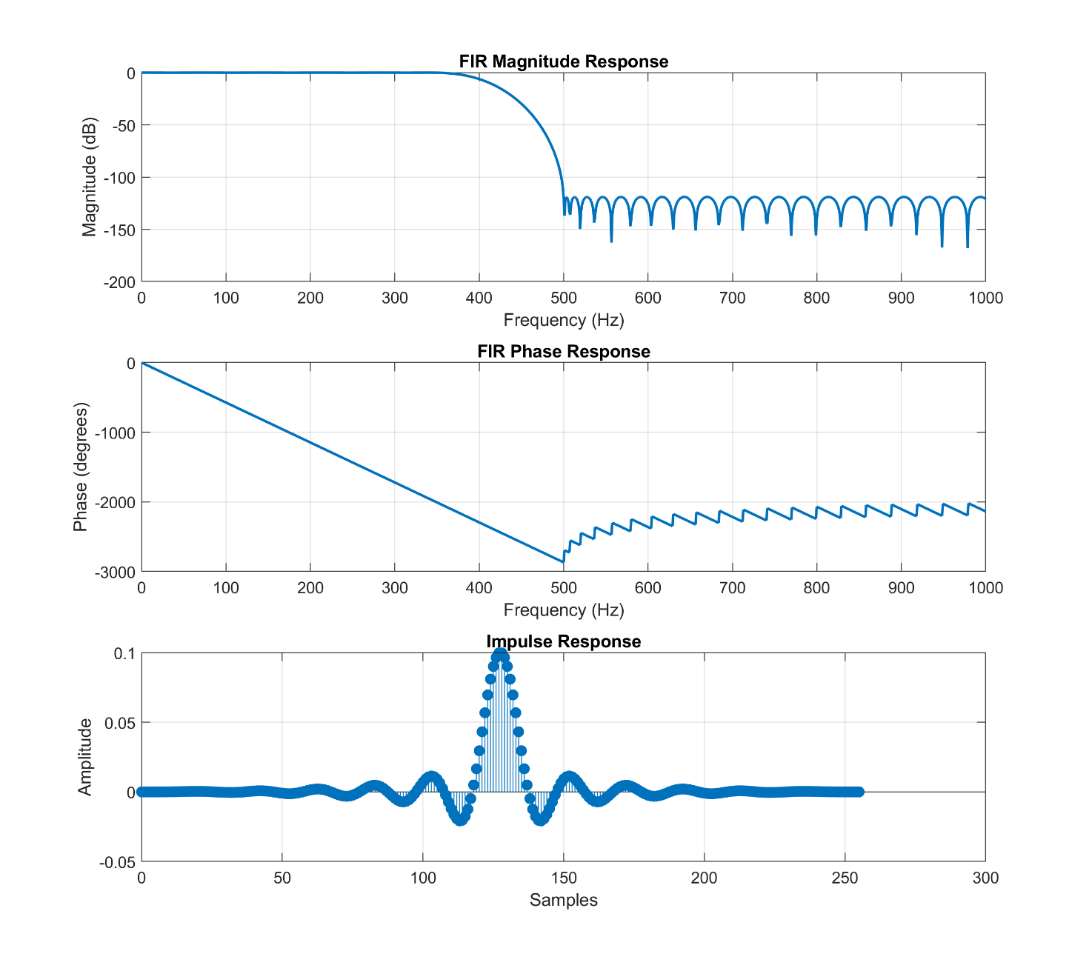Fig. 7A - Frequency response of the anti aliasing filter used for down sampling to 1ksps	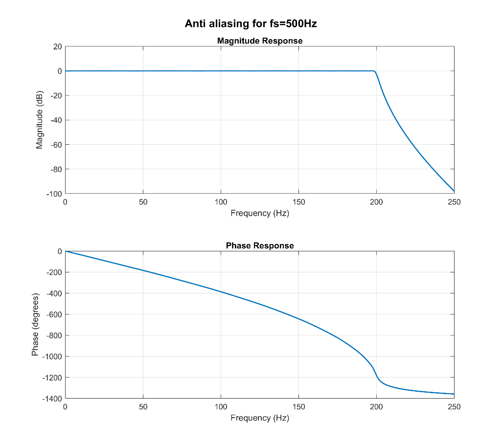Fig. 7B - Frequency response of the IIR anti aliasing filter used for down sampling to 250sps
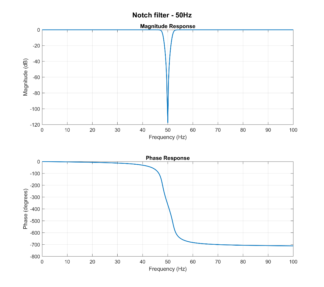Fig. 7C - Notch filters at 50 Hz that can be activated to remove main’s noise	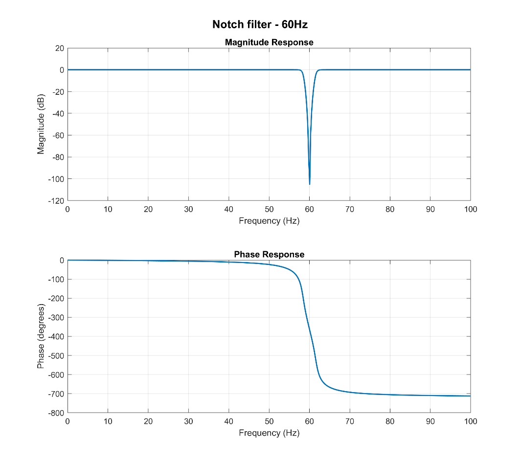Fig. 7D - Notch filters at 60Hz that can be activated to remove main’s noise

Great, We Have the Data… Now What?

All of this is fine—the ADC samples, the data is processed, the filters do their job—but sooner or later an unavoidable question arises: what do we actually do with all these numbers? This turned out to be the main topic of many long (and friendly) discussions with Renato. In the end, we decided to stay faithful to the guiding principle of the project: simplicity. The board was designed to interface directly with Spectrum Lab, a piece of software that anyone working with VLF signals will immediately recognize. It is, for all practical purposes, the Swiss Army knife of low-frequency spectrum analysis. Choosing Spectrum Lab also meant choosing its native data format: the equally legendary 7bitpack, invented by Wolf, Spectrum Lab’s author, specifically for streaming sampled data efficiently. Given our relatively modest sampling rates, the most sensible transport layer was also the simplest one: a plain serial link. On the board, an FTDI USB-to-serial converter handles the interface, making configuration almost trivial and ensuring compatibility with virtually any computer built in the last twenty years—Windows, Linux, macOS… and probably even an Amiga, with enough determination. Data is transmitted at 250 kbps, wrapped in the compact and well-documented 7bitpack format. The most obvious way to use the board is to connect it directly to Spectrum Lab and watch the spectrum unfold in real time. That alone already covers the vast majority of use cases.

That said, the data is not locked into a single ecosystem. I’ve personally experimented with alternative approaches. I’m not a professional programmer, but even I managed to put together a small Python script that reads data from the serial port, writes it to a text file, and periodically converts it into a .wav file. If I can do it, any reasonably motivated tinkerer could probably do the same over a coffee break. I’m happy to share these scripts—though they are admittedly simple, reflecting my status as an enthusiastic amateur rather than a seasoned engineer. Some might see this approach as a limitation: the board does not appear as a native audio device. From another perspective, however, this turns out to be a significant advantage. The humble USB serial COM port is one of the most universal and stubbornly persistent interfaces in the history of computing. It is the cockroach of digital communication standards—it will outlive us all. Audio streaming standards, by contrast, have a habit of disappearing with remarkable speed. FireWire audio interfaces? Gone. ADAT optical multichannel? Mostly gathering dust in studio storage rooms. Betamax, Zip drives, MiniDisc—fondly remembered, rarely used. By sticking with USB serial, the board becomes effectively future-proof. Twenty years from now, when most contemporary audio interfaces are long obsolete, this device will still plug in and work without drama—possibly into a computer embedded in a neural implant.

An eye to the future

That said, we are also exploring a second revision of the design. This future version would use a different microcontroller from the STM family, offering better support for native USB development. The idea under consideration is to implement composite USB functionality: one part of the device would appear as a 24-bit stereo USB audio interface, while the other would remain a communication (COM) device. This approach has clear advantages. It would allow the board to interface directly with a wider range of software, including tools such as Audacity, Adobe Audition, and other general-purpose audio applications. However, it also introduces some drawbacks. For example, Windows does not support USB audio sampling rates below 8 kHz, which means that our carefully designed low-rate acquisition (e.g., 1 kHz) would no longer be directly usable and would require post-processing. At the moment, the idea we are exploring is a hybrid solution. One version of the board could simultaneously:

Output processed data at 1 kHz, 500 Hz, or 250 Hz via the serial interface (fully compatible with Spectrum Lab and custom scripts), and
Provide a raw, unprocessed stereo data stream at 8 kHz, 24-bit, via USB audio.

This ensures backward compatibility while also opening the door to broader software support. The serial interface remains available for precise, low-frequency work, while the USB audio stream enables easy integration with both amateur and professional tools.We are still working on this concept, and nothing is set in stone. For now, we simply wanted to share the direction we’re exploring—and, as always, feedback is very welcome.

The Time Markers: A Simple and Elegant Solution

At this point, all that’s left is to explain in more detail how the issue of temporal markers functions as an absolute time reference. This solution, proposed by Renato, is honestly a solid one and straightforward: from the GPS module to the board, read the usual NMEA strings to extract the exact date and time, and voilà — we know exactly what time it is. Sounds easy — and it is. But what do we do with that information? In more advanced digital audio systems, data packets can carry metadata timestamps embedded directly in the audio stream, often through special modulations, sync signals, or embedded timecodes. You know better than me — professional systems pull off miracles with SMPTE timecode, MIDI timecode, and so on. But we looked at each other and said: “The heart of this project is to deliver excellent performance with simple hardware.” So, we decided to step back in time, to when things were more analog and straightforward — the 1930s, 40s, and 50s — the era of tape recorders. How did they mark time back then? They added a tone, or an impulse, or an offset variation on the analog track. These simple markers had three big advantages:

Visibility: A regular tone or impulse stands out clearly on a spectrogram as bright lines, easily spotted even visually.
Compatibility: No fancy algorithms or complex digital protocols needed; just a variation in the signal that’s easy to isolate later.
Data integrity: Properly set, they don’t wipe out useful data; their duration is so short they’re negligible over hours or days of recording.

That’s the simple approach we chose to solve the timing problem, staying true to the “plug & play” spirit of the board.

How the Time Marker Works on Our Board

We developed a feature called Time Marker. Starting from midnight UTC (obtained for free from the integrated GPS receiver on the board), we can insert time markers at selectable intervals: every minute, hour, two hours, or four hours. Markers sync to the GPS clock with uncertainty tied to the sampling frequency: Precision depends on the marker being inserted at the closest sample to the exact time. What does this mean? Because the system samples the signal at discrete intervals — for example, every 1 millisecond if sampling at 1000 Hz — the exact GPS time we want to mark may fall between two samples.

Since we can only insert the marker at one of the actual sampled points, the marker gets placed at the nearest sample to the target time. This causes a small timing uncertainty, equal to up to half the sampling period. For example: If sampling at 1000 Hz (1 ms per sample), the marker can be off by up to ±0.5 ms from the exact GPS time. At 500 Hz (2 ms per sample), the marker timing uncertainty is ±1 ms. At 250 Hz (4 ms per sample), the uncertainty is ±2 ms. So, the timing precision is limited by the sampling frequency — the faster you sample, the smaller the timing “rounding error” when placing the marker.

Three Ways to Insert a Marker

Users can choose from three modes to insert time markers:

Offset: An adjustable offset from -100% to +100% of full scale is added to the signal and the gain is reduced to avoid saturations. For example, a 10% offset shifts the trace by 10% of full scale; gain is temporarily reduced of the 10% to avoid saturation. So a 50% offset moves the signal halfway to full scale and reduces gain by 50%.
Tone: A 33 Hz sine wave is inserted (the frequency was chosen by Renato after some deep thinking… or maybe chasing a beer, who knows). Tone amplitude is adjustable from 0 dBFS (full scale) down to -80 dBFS.
Constant Value: During the marker, the signal is replaced by a user-defined constant value, expressed as a percentage of full scale for a defined numbers of samples. In this mode, the original signal is temporarily lost, and the output shows only this fixed value for the duration of the marker

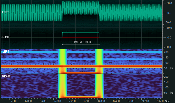
Fig. 8 - OFFSET marker in frequency and time domain. Parameters: Amplitude 50%, length 1s

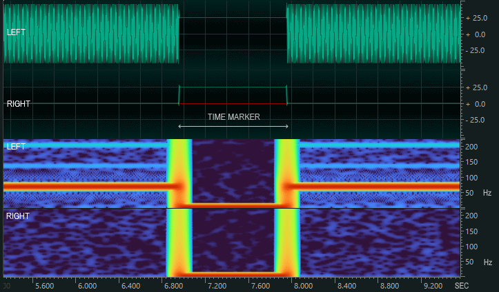
Fig. 9 - CONSTANT marker in frequency and time domain. Parameters: Amplitude 25%, length 500 samples

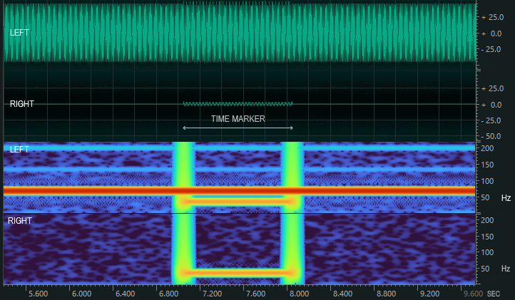
Fig 10 - TONE marker in frequency and time domain. Parameters: Amplitude -30dBfs, length 1000ms

For all three, the marker duration is adjustable: from 1 millisecond up to a second or more, depending on user needs.

It’s simple — no complicated synchronization algorithms, no need for protocol changes or heavy processing overhead. Just straightforward, reliable markers inserted directly into the signal.

It’s practical — these markers stand out clearly in the spectrum analysis, making them easy to spot and use as time references, all without significantly interfering with the actual data you want to capture and analyze.

It’s flexible — users have full control to enable or disable this feature whenever they want, tailoring the behavior to their specific needs and recording scenarios, whether they want precise timing or pure, uninterrupted signal data.

And we’re quite satisfied with this approach because it strikes the perfect balance: it keeps the hardware and software simple, avoids complex timing headaches, and still delivers precise, visible timing markers that anyone can easily interpret. In short, it just works — reliably and elegantly.

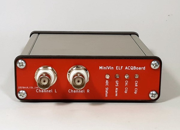
The board

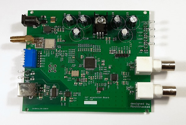
Fig. 11 - Top view of the PCB.

So here we are at the end of this description, where we explained how we reached the current design of this board and what problems we tried to overcome along the way. At this point, the only thing left to do is look at the actual circuit, the printed circuit board, which can be seen in the photograph. The schematic is not particularly complicated, but we took into account and implemented a series of design choices that brought it to a rather industrial level, so to speak, starting with the power supply. The power jack is connected to a TVS for protection, to a diode against reverse polarity, and a fuse to prevent, well, the board from catching fire. Then we have a nice common-mode filter with a common-mode choke and two differential-mode inductors, followed by a set of capacitors for filtering. From there, the power goes to the voltage regulator. As you can see, we didn’t skimp on capacitors. We also mounted smaller capacitors because we changed the enclosure along the way: at first, we could have used 5 cm tall capacitors, but in the final case there’s much less space. The regulator used is a Low Dropout LF33A. We decided against a switching regulator, fearing the kind of garbage and self-induced noise it might produce. So we went with an LDO. The board draws a fair bit—around 160 mA—so it’s best to power it with 5–9 V to avoid turning it into a little space heater. In the next revision, I’m working on a low-noise switching converter… though, as anyone who’s tried will tell you, efficiency, low noise, and affordability rarely like to appear in the same sentence.

Moving on, in the center of the board, under the PIC microcontroller, you can see the the 10 MHz VCXO. Next to the VCXO is IC4, the active filter: a third-order Sallen-Key. On the far right is IC7 is the analog-to-digital converter. You can see the symmetric PCB traces to the inputs, the RC anti-aliasing input filter, a 27 kΩ resistor that sets the input impedance. The front-end has two Zener diodes that protect against voltages greater than ±2 V and against ESD and overvoltage with additional help from the 1 kΩ input resistor.

All data and settings are saved in an EEPROM, which you can spot in the lower part of the board. On the left-hand side there’s a Quectel L76 GPS module — these GPS units directly power the antenna at 3.3V. It is connected to the microcontroller via UART to program the module and to read every second, the NEMA timing strings. Reading the NEMEA strings we can understand if the GPS is traking or not, enabling in this way the GPSDO and the marker structure.

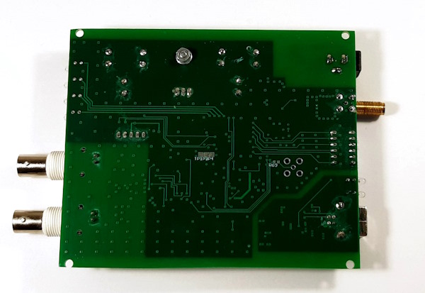
Fig. 12 - Bottom view of the PCB.

Also on that side, you can see a bank of DIP switches for selecting settings (we’ll see how they’re configured later), two LEDs to indicate transmit and receive status, and the USB interface with an FTDI chip. Notably, to avoid injecting noise into the board, this section is fully isolated — if you look closely, you’ll see the USB area has no top ground plane. IC2 is the chip that provides galvanic isolation for TX and RX signals, preventing all the noise and junk coming from the processor from reaching the acquisition board, thus keeping the signal clean.

On the front panel, there are the two BNC connectors for the input signal and some LEDs indicating whether the input is clipping, whether the GPS is in “alarm” state because the antenna is missing or it’s not traking any satellites, and the “DC Status” LED showing whether the system is running in free-running mode or locked to the GPS, synchronized UTC time with the markers and all that stuff.

Board Configuration via DIP Switches

To wrap things up, I’m not going to bore you by explaining the meaning of every blink of every LED. Still, it might be useful to give you an idea of what you can do with this board without too much effort. On the back of the board there are 6 DIP switches used to configure the operating modes of the device. The switches are numbered from 1 to 6, and the ON position corresponds to the lever pointing downwards (as marked on the switch body).

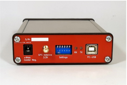
Fig. 13 - Minivin Rear side

1. Sampling Frequency

Set the desired sampling frequency according to the following table:

Sampling Frequency	DIP2	DIP2
1 ksps	OFF	OFF
1 ksps + 50/60 Hz notch filter	ON	OFF
500 sps	OFF	ON
250 sps	ON	ON

Note: The notch filter frequency (50 Hz or 60 Hz) can be selected via configuration software that we will present later

2. ADC Gain (PGA)

The ADC is preceded by a Programmable Gain Amplifier (PGA), which allows adjusting the input gain in hardware before digitization. This PGA is chopped-stabilized, meaning it does not exhibit flicker noise and shows a almost flat noise spectral density at all frequencies.

With unity gain, the input dynamic range is approximately 1 Vpp. Increasing the gain reduces the available input range.

Sampling Gain	DIP3	DIP4
×1	OFF	OFF
×4	OFF	ON
×8	ON	OFF
×32	ON	ON

3. High-Pass Filter for AC Coupling

The ADC normally digitizes from DC (direct coupling). However, it is possible to enable a high-pass filter to remove the DC component.

By default, this filter is set at 10 Hz, but its cutoff frequency can be changed via the configuration software between 362 Hz and 19 mHz. Remember that this filter is implemented digitally into the ADC firmware. If the ADC input saturates before filtering (for example, due to excessive DC offset), the saturation will still corrupt the data despite the high-pass filter being enabled.

Coupling Type	DIP5
AC Coupling	ON
DC Coupling	OFF

4. Calibration Signal

The last DIP switch allows you to disable the ADC and generate a calibration signal at 33 Hz. This mode is useful for verifying correct configuration in SpectrumLab or similar analysis tools.

Function	DIP6
Calibration signal ON (33 Hz)	ON
Normal ADC operation	OFF

Configuration program

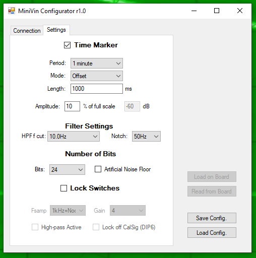
Fig. 14 - View of the configurator. Here you can see all the configuration that you can perform on this acquisition board

For more advanced use, you can connect the board to a computer via USB and configure it with a small utility we’ve developed. This program gives you access to all the adjustable settings we decided to keep variable: whether the time marker is enabled or not, the time marker period, the operating mode, the high-pass filter frequency, the notch filter frequency (50/60 Hz), the bit depth (16 or 24 bits), and so on.

And if the board needs to be installed somewhere remote and out of reach, you can lock in a precise configuration and disable the switches altogether. That way, no one can tamper with the unit or set the switches in an unintended way. Another practical advantage is that this configuration tool uses the same USB cable as the data stream. If the board is connected to a distant or hard-to-reach computer, you can simply start a remote session, open the program, and adjust the settings from wherever you are. The program does have one significant limitation: if multiple boards are connected to the same computer, at present it will only communicate with the board that has the lowest COM port number. We know this is a shortcoming, and we’ll fix it if — or rather, when — someone actually needs it solved.

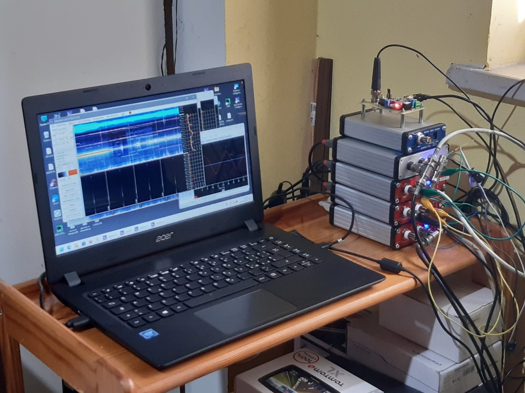
Fig. 15 - We don't know if any of you will ever need to connect 4 MiniVins to the same PC.
But if you do... know that it works, and with minimal use of PC resources.

So, here we are — some tests on the stuff.

So far, we have described how the board works, the challenges we set out to address, and the strategies we adopted. At this point, however, we cannot yet claim complete success—but by the end of this section, the results will speak for themselves. Before diving into the inner workings of each LED or configuration detail, we decided it would be more illustrative to perform some measurements. As a baseline, we compared our MiniVin acquisition board with my Sound Blaster SBX, model SB1095. The simplest initial test was to feed both devices with the same signal: 400 mV RMS, generated by a Siglent SDG2042X function generator. A simple test, perhaps trivial in setup, but it already revealed significant differences. The MiniVin captures the signal almost exclusively along with its second harmonic, while the Sound Blaster picks up additional components at 50 Hz, as well as intermodulation products between the 50 Hz and the main signal.

In other words, the Sound Blaster exhibits a noisier, less clean response, despite identical cabling and signal source. The explanation is likely related to isolation. The MiniVin communicates with the computer via a galvanically isolated, opto-isolated USB link, while the Sound Blaster does not. As a result, the latter is prone to ground loops and interference from the USB bus itself, introducing additional noise. Another notable difference lies in bandwidth. The MiniVin’s bandwidth is intentionally limited to approximately 350–360 Hz, whereas the Sound Blaster remains clean up to nearly 500 kHz.

This is due to fundamental architectural differences: Windows and the Sound Blaster do not support a 1 kHz sampling rate, so the card samples at its maximum rate, 48 kS/s, and the downsampling is handled in software (Spectrum Lab), which effectively stretches the observed bandwidth. In contrast, the MiniVin truly samples at 1 kS/s, with careful attention to aliasing, which imposes the observed bandwidth limitation. This constraint can be advantageous or restrictive, depending on the application. Dynamic range is another point of contrast. The Sound Blaster exhibits a signal-to-noise ratio approximately 10 dB higher than the MiniVin. Nevertheless, the MiniVin achieves superior performance in terms of SNR.

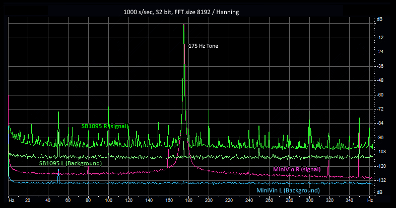
Figure 16A - Same 175Hz - 400mVrms signal recorded with miniVin and SB1095 shown in the frequency domain: spectrum and waterfall view.
On the MiniVin, we observe that the background noise on the free channel is much lower than on the sound card.

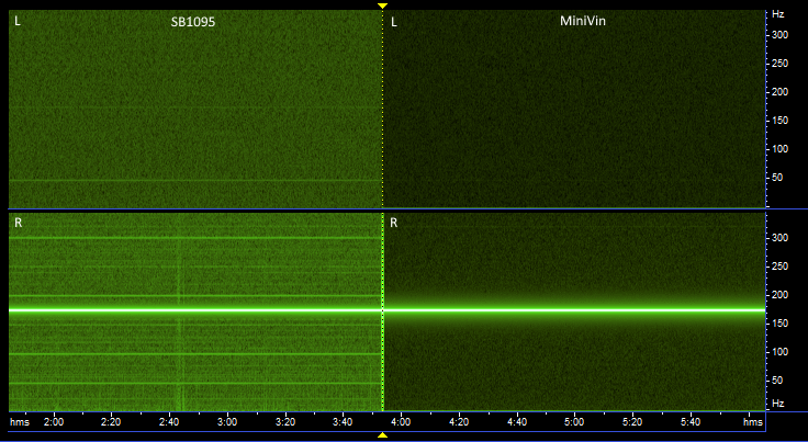
Figure 16B - Furthermore, there are fewer artifacts created on the signal arriving from the function generator:
this is due to the ground loop created with the sound card, which is not present with the MiniVin.

These differences become even clearer when examining the noise spectral density. A comparison plot highlights the roughly 10 dB advantage of the Minivin across the frequency band. Additionally, the Sound Blaster shows the characteristic 1/f noise rise at low frequencies, even with AC coupling, whereas the Minivin maintains a predominantly flat noise profile. These measurements were made with a high-pass filter set at 77 mHz, in combination with unity gain, which maximizes the flatness of the noise spectral density. It is worth noting that if DC coupling were used instead, the low-frequency noise would gradually rise toward DC. This effect is expected: the 1/f noise reflects, in a sense, the incipient random walk of the internal reference—the unavoidable drift of the signal over time. Sigma-delta converters minimize this effect, but they cannot eliminate it entirely. Complete suppression would require a global chop mode architecture to cancel the low-frequency drift as much as possible. We are currently exploring the GlobalChopMod, and it is not impossible that, in a future revision of the hardware, if this approach proves effective, it could be integrated directly into the board. The goal would be to achieve truly precise measurements down to DC, effectively eliminating any residual drift in the system. For now, however, the results are already clear: the MiniVin shows a decisive advantage over the Sound Blaster. We also examined the noise behavior as a function of input gain. With a gain of x1,x4, x8 and x32, scaled accordingly, the results are telling: for each increase in gain, the background noise decreases proportionally. What does this imply? Essentially, it indicates that the input stage of the Minivin contributes negligible noise to the overall system. In other words, the measured system noise is dominated by the ADC itself, rather than the preamplifier or input electronics. This confirms that the board’s analog front end is well-designed and sufficiently quiet, allowing the sigma-delta ADC to define the ultimate noise floor.

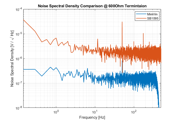
Fig. 17 - Noise spectral density: MiniVin vs SB1095. MiniVin settings: 1ksps, HPfilter: 77mHz, unitary gain.

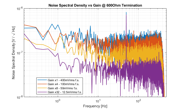
Fig. 18 - Noise spectral density of MiniVin. Settings: 1ksps, HPfilter: 77mHz, gain x1, x4, x8 and x32.

So, what have we actually achieved with this board? Is it just another small circuit, or something approaching the performance of a professional data logger? Our goal was to create an affordable device, technically capable of handling a wide range of monitoring tasks, while remaining user-friendly, compatible with free software, and requiring no programming knowledge. The proof of this approach is illustrated in the following spectrogram, generated using Adobe Audition The results are striking: signals at tens of millihertz, entirely invisible to a standard sound card—such as teleseisms and geomagnetic pulsations—become accessible.

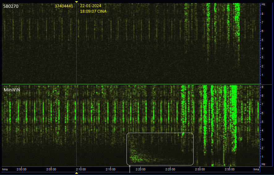
Fig. 19 - An earthquake occurred in China, thousands of kilometers away from Italy detected with a vertical geophone.
The time of the earthquake is indicated by the dotted yellow line.

With nothing more than a simple PC and a session of Spectrum Lab, one can acquire data that meets research-grade standards, suitable even for advanced studies and publications. As an example, the figure shows an earthquake that occurred in China, thousands of kilometers away from Italy. The dashed yellow line marks the moment of the earthquake. The highlighted rectangle shows the seismic wave as it arrives in Cumiana, Italy, where our geophone recorded the signal. In the top panel, the same geophone output was acquired by a Creative SB-0270 sound card, connected in parallel with the MiniVin. The seismic signal is not visible, lost in noise. In contrast, the bottom panel shows the same signal acquired by the MiniVIN: clearly visible, well above the noise floor, and fully discernible. We felt that this measurement—with real signals under real conditions—demonstrates the instrument’s value far more than countless technical bench tests. It shows, in practice, the effectiveness and performance of the device for scientific monitoring.

Here is another example of reception with a MiniVin card, where you can see a signal that you would never see with a sound card: a teleseism.

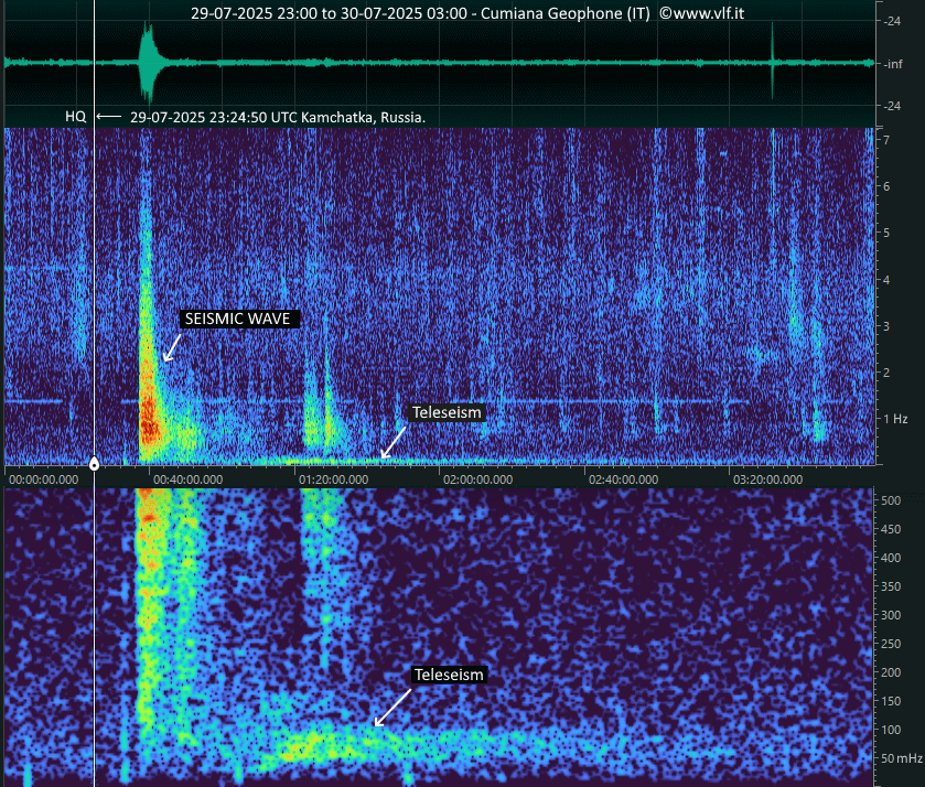
Fig. 19 -The spectrogram shows 4 hours of reception with a geophone. The seismic wave received in Italy from an earthquake in Kamchatka, Russia, is clearly visible. However, a teleseismic event triggered by the phenomenon is also evident, with a signal lasting several hours, around 50 mHz.

Thank you for your attention!

Final Note

A final, and rather delicate, note — so I’ll tread carefully here. This board, and indeed this entire article, is being published on www.vlf.it, a site we all know as a place for open sharing — independent, ad-free, and sponsor-free. It’s run by the remarkable Renato Romero, who earns nothing from it — in fact, he likely invests his own time (and perhaps even money, though I’ve never dared to ask). In keeping with the site’s spirit of sharing, you’ll find at the end of this article a single zipped package containing the complete schematic, the BOM, the Gerber files for PCB manufacturing, and the compiled .hex file for loading into the microcontroller. We do, however, recognise that this is not exactly the most beginner-friendly or instantly buildable of projects. For that reason, should there be interest from more than one person in owning a board — and since we’re already planning to produce a small batch for Renato’s station — it would make sense to hear from you. If enough people come forward, we could consider producing a larger quantity, which would naturally lower the overall cost per board. A saving for everyone, in other words.

Download the zipped package from here: ACQBoard_Docs_rev2.zip

Return to www.vlf.it home page