AND VISUALIZATION ON POLAR MAP
By Valerio Cammelli
To correctly represent the azimuth of a spheric on a map it is necessary to have the two components NS-EW of the H field of the two loop antennas and the vertical component of the electric field EZ, refer to the previous article regarding the details of the magnetic antennas and the acquisition of the channels (ref.1, Tweeks and sferics distance calculation).
The following topics will be developed:
1) Antenna for electric field and EZ signal processing
2) Principle of determination of arrival azimuth with two crossed loop antennas
3) Quadrant determination via signals NS, EW, EZ
4) Determination of the radial and transverse components.
5) Recording of waveforms NS, EW, EZ
6) Processing of NS, EW, EZ signals and azimuth determination
7) Spheric Waveform example
8) Polar map representation of the strike
9) Magnetic and electric antennas setup
10) Validation of the method with comparison with Blitzortung.org
11) Conclusions
12) Bibliography
1) Antenna for electric field and EZ analog signal processing
This antenna was built following the project of I1RFQ Claudio Re “ADA an active differential antenna for 5Hz-500 KHz “on www.vlf.it (http://www.vlf.it/cr/differential_ant.htm). It consists of two aluminum pipes mounted vertically on a support consisting of a short plastic tube 10 cm long.
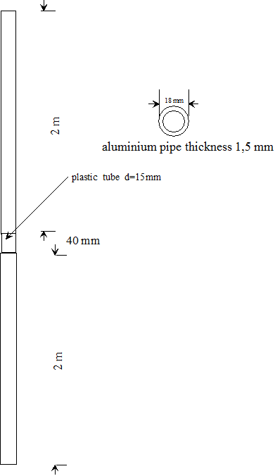
Fig.
1 Vertical antenna for electric field
The gain of this antenna was evaluated according to the criteria reported in the article “Notes on dimensioning a minima electrical field receiver for ULF/VLF bands of Andrea dell'Immagine on www.vlf.itwith the following values :
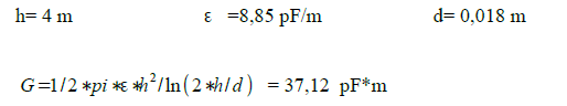
The sensitivity of the antenna is thus comparable to the magnetics antennas already described in the previous article. The receiver scheme (fig.2 and 2_1) differs from that of I1RFQ: the instrumentation amplifier made with 3-op amp has been replaced with a monolithic instrumentation amplifier, AD620.
An RC Band-pass filter has been inserted to limit the noise in the 1 to 22kHz band of interest, follows a double T active notch filter centered on 50 Hz since the 50Hz noise that is coupled to the antenna was very high. The notch filter output is converted into digital by the USB-204 DAQ MC and then processed with the Labview RX-lightning .vi sw program on the PC.
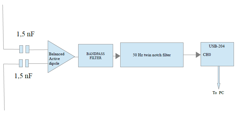
Fig.
2 RX and EZ signal processor
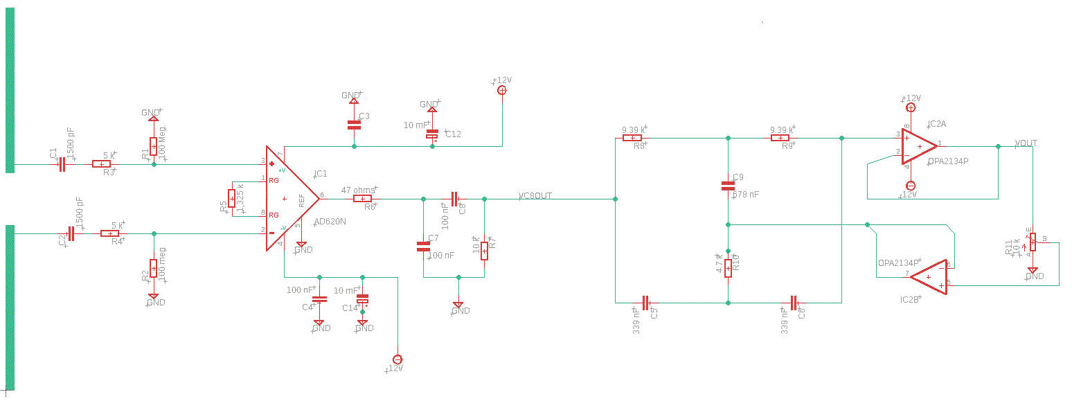
Fig.
2_1 electric scheme RX E Channel
Fig. 3
Antenna for electric field
2) Principle of determination of arrival azimuth with two crossed loop antennas
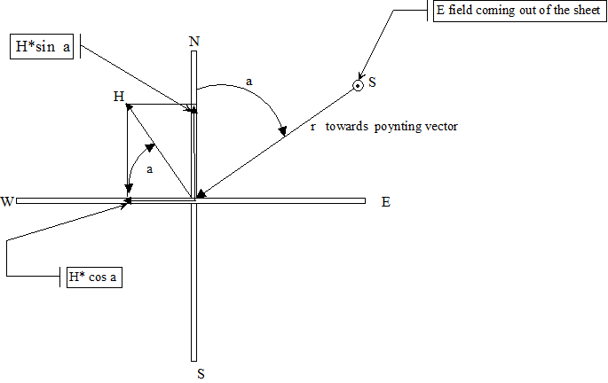
Fig.
4 Horizontal view of the two antennas
The two ortogonal antennas are shown in fig. 4 (projection in the horizontal plane).One is oriented in the NS plane the other in the EW plane. The source S is the vertical field E which excites mainly the TM Mode (transvers magnetic) (ref.5). The angle with the north direction is a.The field H is therefore perpendicular to the direction of propagation r with angle a with respect to N.
The flux of the magnetic field H in the S vertical section of the NS antenna consisting of N turns will be:
The time-varying flux induces a f.e.m. :
similarly for the EW antenna :
The ratio between the two waveforms:
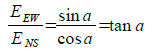 from which the angle :
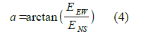
in the theoretical case of a sinusoidal magnetic field H with pulsation w the (2) e (3) turns :
Y(t) = Va* Sin (a)* Cos(wt) (5)
X(t) = Vb* Cos (a)* Cos(wt) (6)
we put the waveforms (5) e (6) in a XY graph
we obtain two possible straight lines ss' or ss:
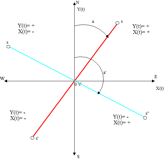
Fig.
4a phase x(t) an y(t) in the four sectors
if y (t) and x (t) are sinusoidal waveforms of the same frequency and with zero phase shift (fig.5 and 6), a straight line segment will appear in the XY graph, included
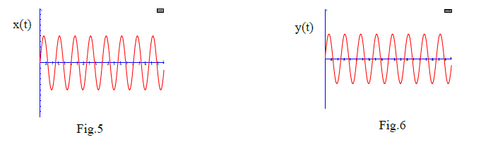
within the NE quadrant with angle of inclination a with respect to North (figures of Lissajoux). Since (4) gives the angle a with an ambiguity of 180 degrees, the half-straight part Os' is also a solution of (4), with waveforms in phase but with negative initial amplitude: fig. 7 and 8.
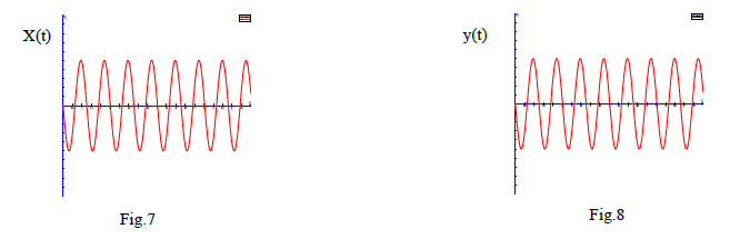
For an angle a' belong to the NW and SE quadrants (straight ss"), y (t) and x (t) will be out of phase by 180 degrees, precisely in the NW quadrant y (t) will have positive initial amplitude while x (t) will be negative .In the SE quadrant the opposite will occur. The correct signs of y (t) and x (t) in the four quadrants are shown in fig.4a.
In the real case the waveforms are not sinusoidal and the fields are not linearly polarized,so instead a straight line as in fig. 4a we will have an ellipse
3) Quadrant determination via signals NS, EW and EZ
Knowing the signs of the initial amplitude of y (t) and x (t) we obtain the quadrant of origin of the lightning.
This is true if the electric field of the stroke always has the same polarity, in most of the strokes the discharge is negative (-CG) therefore by convention the electric field is positive (EZ +) but in about 10% the discharges is positive + CG (ref. 4) and therefore the vertical electric field is negative (-EZ)
In this case the source will be 180 ° from the sector indicated by the sign of x and y.
In fig. 9 let S be the source of the lightning stroke in the NE quadrant, the positive electric field Ez comes out of the plane in figure 9, the magnetic field H (mode TM) is perpendicular, the poynting vector will be directed towards the observer O according to P = Ez x H.
where x stands for vector product and P is the poynting vector. The direction of P is easily determined with the right hand rule applied to the vectors Ez and H.
Now suppose that in S the stroke is + CG (Ez-) applying the previous rule we see that the vector P is not directed towards the observer, this cannot be.It is easily sees that the right solution is the source in the quadrant SW, in fact maintaining the same components of H and applying the right hand rule with (Ez -) the vector P is directed towards the observer.
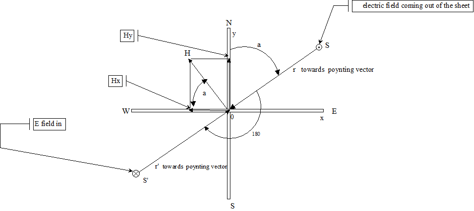
Fig.
9 Electric Filed and pointing vector
So the rule is this: if the electric field has a positive initial amplitude, the sector is determined by the signs of the initial amplitudes of Y (t) and X (t) as shown in fig.4a, if Ez is negative, 180 degrees is added to the azimuth a.
4) Determination of the radial and transverse components.
The real spherics are'nt juste TM modes but there is also the TE mode (electrical transverse), indeed in correspondence with the 1.8 Khz cut-off frequency the QTM1 mode is more attenuated than QTE1 ,so we have a mix of the two modes, TM is responsible for the Ht component transverse to the propagation direction and TE for the radial Hr component.It is therefore advisable to calculate both and use the one that has the greatest amplitude.This component Hr from TE mode is in quadrature with Ht and it is responsible for the elliptical polarization of the spheric and for the azimuth error (ref. 7). We do not consider this problem for now, but we must bear in mind that this error increases when the angle of incidence of the wave with respect to the horizontal plane upgrade.
Referring to fig. 10 with the source S in sector NE, the magnetic field H , not perpendicular to the r direction is decomposed into Hew relative to the antenna EW and Hns relative all'antenna NS, these components are broken down into Ht transverse to the r direction and Hr radial .
Ht = Hew*sin a + Hns*cos a (6)
Hr =Hew*cos a – Hns*sin a (7)
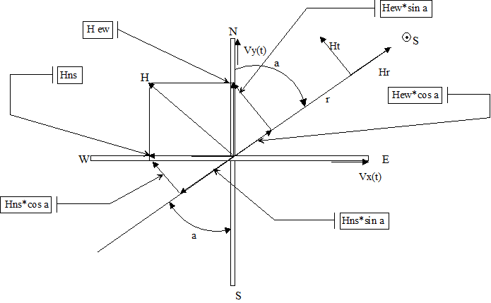
Fig.10 radial and transverse component
but Hew ~ Vx (t) because the magnetic field Hew induces the voltage Vx in the EW antenna and Hns ~ Vy(t)
Thus (6) and (7) become :
Ht = Vx(t)*sin a + Vy(t)*cos a
Hr = Vx(t)*cos a – Vy(t)*sin a
For the source in the SW quadrant we have, as
sin(a+180) = -sin a
cos(a+180) = -cos a
Ht = -Vx(t)*sin a - Vy(t)*cos a
Hr = -Vx(t) *cos a +Vy(t) *sen a
For the source in the SE sector we have :
Ht = Vx(t)*sin a - Vy(t)*cos a
Hr = -Vx(t) *cos a +Vy(t) *sin a
and for the NW sector: since a => a+180
Ht = -Vx(t)*sin a + Vy(t)*cos a
Hr = Vx(t) *cos a -Vy(t) *sin a
5) Recording of NS, EW, EZ waveforms
In order to identify the direction of arrival of the spherics and to compare it with the data from Blitzortung.org, it was necessary to develop a program in labview that would allow the simultaneous recording of the three afore mentioned waveforms.This recording is possible in real time with representation on the polar map and on command with storage of the waveforms on hard disk.
The file name for each recorded waveforms was set like this:
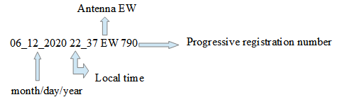
Two other files are similar for recording from the NS and EZ antenna with the same progressive registration number.
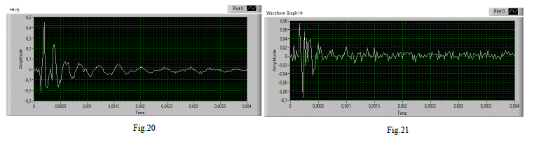
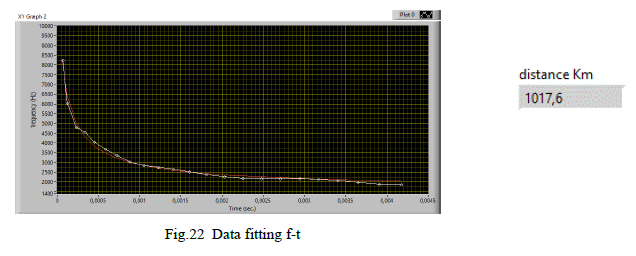
Another program: "spheric XYZ reading without filters.vi" is able to recover all three files of the same progressive number to process them and obtain the azimuth and the Ht / or Hr components from which the algorithm presented in the previous article (rif.1) calculates the distance.
6) Processing of NS, EW, EZ signals and azimuth determination
The block diagram is shown in fig. 11.
The operator selects the EW XXX file and automatically the three files EW, NS, EZ are read, the program shows the three waveforms. The sign of the first peak of the signal EW and NS together with the sign of EZ determines the quadrant of origin of the spheric.
The EW and NS signals are plotted in an XY graph (point graph) to which a labview function is applied: linear fit that approximates these points with a line obtained with the minimum distance squared method. The slope of this line is the azimut with ambiguity of 180 degree.With the information of the signs of EW, NS and EZ it is possible to eliminate the ambiguity of 180 of the azimut and position the origin of the spheric. With the angle a and the quadrant of origin, the Hr and Ht are calculated with the previous formulas .
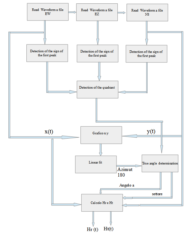
Fig. 11 Azimuth
and Ht, Hr determination
7) Spheric Waveform example
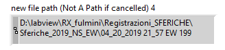
Fig.12
file path of sferic 199
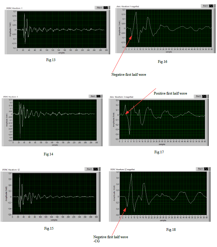
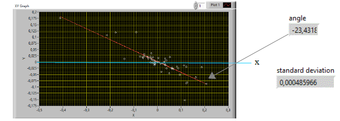
Fig.19 XY
plot of NS e EW and linear fit
The figure 12 represents the file path of the spheric example, in our case it refers to a spheric received the day 4-20-2019 at 21.57 local time with progressive number 199.The components of this spheric are shown in figs. 13,14,15, which respectively represent the components NS, EW, EZ. The duration of the spheric has been standardized to 6ms corresponding to 300 samples, indeed with ck A / D = 48 Khz we have 300 * 1/48000 = 6.025 ms.
In figs. 16, 17, 18 the first 60 samples of the spheric are shown to highlight the phase relationship between the components and also to minimize the polarization error in the azimuth determination (ref.6).
In fig. 19 the XY graph of the waveforms in fig. 16 and 17.The red line represents the line that best approximates the data with the least squares method. The labview function measures the slope of the line with respect to the x axis which is -23.43 degrees (+- 180) and the standard deviation.
From the waveforms of fig. 16 and 17 it can be seen that the first half wave is negative for NS and positive for EW, the sector of origin would therefore be SE (see fig. 4a) but being EZ negative for what has been said previously, the sector is opposite: NE, the angle to the north is therefore:
90 + 23,43 + 180 = 293,43 N
8) Polar map representation of the strike
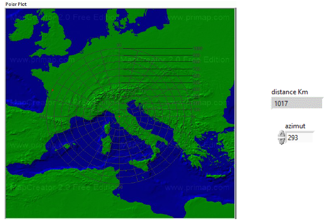
Fig.23
polar map
Once the azimuth and distance coordinates of the strike have been obtained, these can be displayed on a polar map generated by a labview program as shown in fig. 23
9) Magnetic and electric antennas setup
Since the phase of the waveforms is any a priori, it is necessary that they have the right phase to match the real situation to the conditions of fig. 4a.
Electric antenna: it is necessary to discriminate between the discharges + CG and -CG, it is necessary to choose a day in which there are disturbances far enough away > 500 km (check with Blitzortung.org), then recording the spherics you will have to make a statistic: the discharges more frequently they are - CG (Ez + field), the less frequent ones + CG, if this is not the case, it is necessary to invert the antenna wires or invert the signal at sw level.
Magnetic antennas: with a perturbation with d > 500 km and located in a single quadrant (e.g. SE) (check with Blitzortung.org) acquire the NS, EW, EZ channel and check the signs of the first waveform peak that they must be as in fig.4a if EZ is positive: (NS- and EW +).If this is not the case, invert the wires of the NS and / or EW antennas to obtain this result (alternatively invert the signal at the sw level).
10) Validation of the method with comparison with Blitzortung.org
The blitzortung.org website maintains daily historical data of lightning maps up to November 2015 at intervals of 10 minutes.These data are freely available on the site in the historical data menu and can be used to make comparisons and validate the results obtained with the method of of the single station described above.
In particular, in correspondence with our registration example of 04-20-2019 at 21.57 local time blitzortung shows:
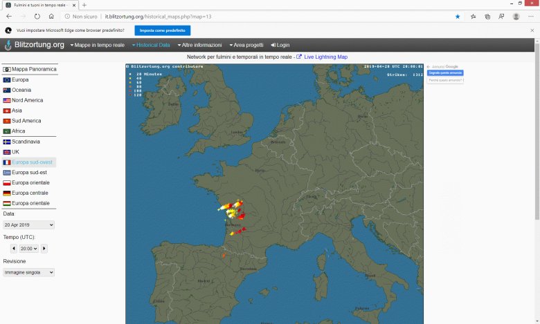
Fig.24
map of Blitzortung.org with lightning activities april
20 2019 at 20 UTC
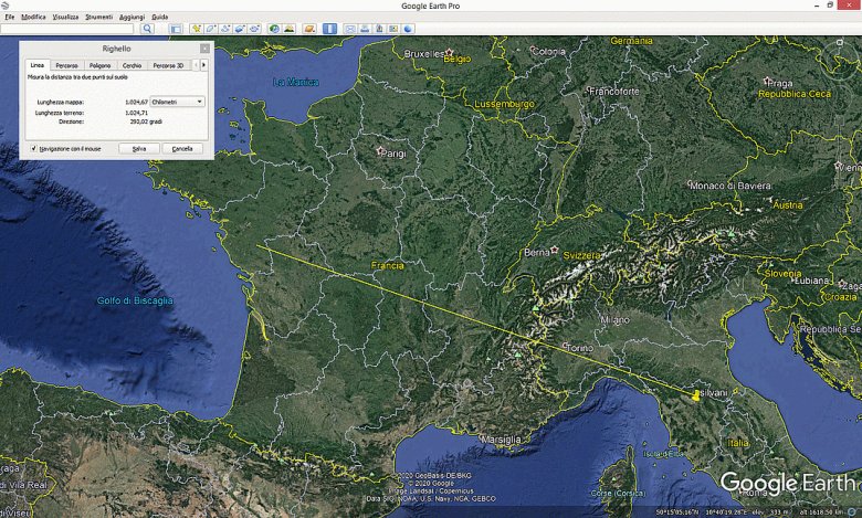
Fig.25
Google Earth map with distance and azimut of sferic
2019 april 20 at 21,57 UTC n.199
In fig. 24 note that UTC 20.00 has been selected for the date 04-20-2019; indeed we have the relation: UTC time = Local time-2h to take into account the time zone and DST.
Fig. 25 shows the Google Earth map by setting the azimuth and the distance obtained in the previous example.
The correspondence, as you can see, is good.
11) Conclusions
An antenna for vertical electric field with sensitivity equivalent to the magnetic antennas already described and a practical method to identify the correct azimuth of a spheric / tweet, taking into account the information of the three antennas, was presented.
Together with the determination of the distance of the spheric developed in the previous article
(ref. 1) this allows you to position the origin of the spheric in a polar map.
A comparison was made with the historical data of Blitzortung.org highlighting a good correspondence.
Of course we cannot expect great accuracy from a single station, professional methods or the Blitzortung.org network itself use a large number of stations.The method is limited to + -CG discharges with good quality spherics and at distances > 500 km , the accuracy of pointing to the north and east of the magnetic antennas together with the polarization error that can reach tens of degrees it is the main limitation.
12) Bibliography
1) Tweeks/sferics distance calculation by V. Cammelli nov.2018 www.vlf.it.
2) VLF Notes Paul Nicholson 2018-04-02
3) ADA an active differential antenna for 5Hz-500 KHz “ Claudio Re su www.vlf.it.
4) Lightning: Physics and Effects Di Vladimir A. Rakov, Martin A. Uman pag.4-6
5) Modal Phenomena in the Natural Electromagnetic Spectrum Below 5 kHz
Dana Porrat∗Peter R. Bannister†Antony C. Fraser-Smith
Radio Science Volume 36, Number 3, Pages 499-506, May-June 2001
6) Accurate and efficient long-range lightning
Geo-location using a vlf radio atmospheric Waveform bank
Ph.D. thesis, Stanford University,Said R. 2009 pag.76
7) VLF goniometer observation at halley bay, antarctica-1.
The equipment and the measurement of signal bearing.
K. BULLOWGII and .J, L. SAGREDO*
Department of Physics, University of Sheffield, Sheffield S3 7R.H, England
Planet. Space Sci. 1973, Vol. 21, pp. 899 to 912
Thank to Alan Melia (G3NYK) for the english corrections .
Return to www.vlf.it home page