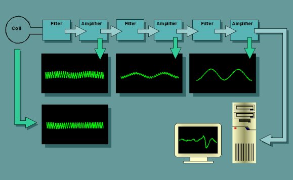
Schematic diagram of the ELF-Receiver: The 50 Hz hum gets, stage by stage, more and more suppressed.
The signals below 50 Hz get, stage by stage, more and more amplified.
On this web page, the author tells about his experiences in receiving ELF waves in a frequency range between zero and approximately 25 Hz. Normally, this range should be completely free of signals, except those from the 16 Hz railway supply, the Schumann Resonance and a few natural signals, caused by solar activities. But to the author's surprise, a number of obviously artificial signals seem to be sended out by some unknown sources permanently, created by electric currents flowing through the surface of the ground and only visible and hearable by using a sound card as a kind of "time microscope".
A little bit of history
Since my youth, I was enthusiastic about shortwave communication (frequencies between 2 and 30 MHz). In the early nineties, I got interested in receiving VLF signals when I learned about natural atmospheric signals, such as "sferics". So I built my first self-developed receiver for frequencies between a few hundred Hertz and approximately 10 kHz.
Though the electronic circuit of the receiver worked successfully, the so-called "whistlers" I received were disturbed by the 50 Hz hum surrounding us everywhere, which is the frequency of mains power in Europe. In spite of sophisticated electronic filtering circuits, the hum could not be suppressed because of the great number of harmonics it contains.
Why use a receiver for less than 50 Hz ?
Only in theory, this hum is sinusoidal. In reality, it is not only distorted by all those machines driven by electrical power, but also by the complex wiring of our mains systems. These distortions create harmonics at multiples of 50 Hz, i.e. 100 Hz, 150 Hz, 200 Hz, 250 Hz etc. up to the kHz-range: Exactly the range I intended to explore was distburbed by these harmonics.
In addition, the 50 Hz hum exists almost everywhere: not only in houses, but also out in nature. This is because the currents going back from the consumer loads to the power stations are partly using the natural ground as a conductor. Besides, all those high-voltage power lines crossing fields and forests are radiating the 50 Hz signal in a strong way.
Facing all these problems, I decided to give up this frequency range and taking a closer look at frequencies below 50 Hz, the ELF range. As harmonics only exist above and not below the basic frequency of a signal, there wouldn't be any disturbances below 50 Hz. But which natural signals could I expect in this range? Officially, there is no commercial or military communication below 50 Hz – but in this range, you also can find signals similar to sferics and produced by natural processes in the atmosphere – especially at periods of sun spots and polar lights.
So I built a voltage amplifier with an amplification factor of approximately 240000 and a low-pass filter with a transfer function of 36 dB per octave and a cut-off frequency below 50 Hz. This may sound complicated, but by using modern operational amplifiers it is a very easy task for an experienced electronic amateur.
For the antenna, I used a self-made coil of 1000 turns and a diameter of 0.4 meters. The idea, to do it just this way and not otherwise was more a question of intuition than a question of investigation: I did not know any source of literature dealing with this topic.
Schematic diagram
of
the ELF-Receiver: The 50 Hz hum gets, stage by stage, more and
more suppressed.
The signals below
50
Hz get, stage by stage, more and more amplified.
First testing results
After the cirquit was built up, I testetd it with a slowly running oscilloscope and a magnet, extracted from an old car loudspeaker. The result was phantastic: Even at a distance of 10 meters, the oscilloscope reacted with a clear and full range sine-like waveform when I slowly moved the round shaped magnet (diameter 6 cm) with my hand. With small metal objects like keys and screw drivers I got the same results if the distance was reduced to a maximum of two or three meters. Passing cars on the street (distance more than 20 meters) with their big metal masses resulted in clipping the signal on the oscilloscope screen.
But even when I located the coil antenna next to an electrical wire, there was no detectable 50 Hz disturbance. This was a proof, that the filter worked perfectly. And even in spite of the high amplification, there was no noise in the signal: If the magnet wasn’t moved and no car passed by, the oscilloscope only showed a straight horizontal line on its screen. But are there no other signals in this frequency range but the ones created by passing cars and moved magnets or metal pieces?
Only a long-time test would bring the answer to this question. So I fed the output signal of my receiver to the input of an analog/digital converter implemented in my personal computer. Additionally, I wrote a program in C running under DOS, which automatically stores the signals on harddisk. At the same time, the signal is shown on the PC screen in the same way it is done by an oscilloscope. To avoid even a small rest of 50 Hz disturbances, the signal is sampled at exactly 50 Hz. According to Shannon, signals up to 25 Hz can be stored on harddisk.
Sampling and saving data
Until today, I performed data acquisition approximately 2 or 3 days a week. The files (limited to a size of 48 kilobytes [16 minutes] due to the DOS memory management) are joined together under Windows and analyzed with a spectrum analyzer software. As this software expects a minimum sampling rate of 8 kHz, the files sampled at 50 Hz are played back 160 times faster. So, the unhearable frequency range below 25 Hz is shifted into a higher, hearable range. This is a great advantage, because the human ear is still a much better analyzing system then any known software. Another advantage of this acceleration is the fact, that long time signal structures which in real time only appear like random can be recognized and detected very easily.
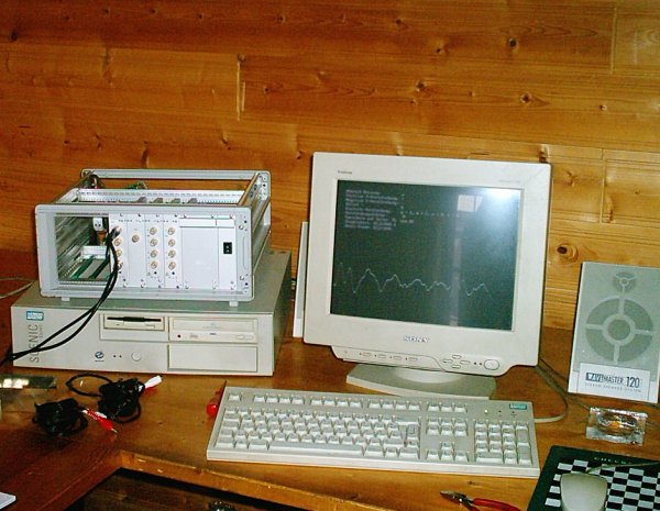
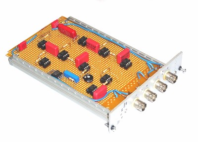
Analog
ELF-receiver
with connected PC and screen, showing a signal of type 2.
Summary of results
The results of these Investigations are very
intersting
and strange. Here a brief summary of what I found out. Obviously
each day,
at irregular hours, a number of strange signals could and can be
received,
which may be categorized in the following way:
Signal
Type
1
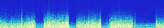
A noise pattern which consists of a noise
period
of 20 seconds and a silence period of 10 seconds (realtime).
Groups of
this pattern, consisting of a constant number of noise/silence
units are
often interrupted by a longer constant period of silence. So,
any natural
origin can be excluded. Played back at 160 times the original
speed, it
sometimes sounds like an old-fashioned steam-powered locomotive.
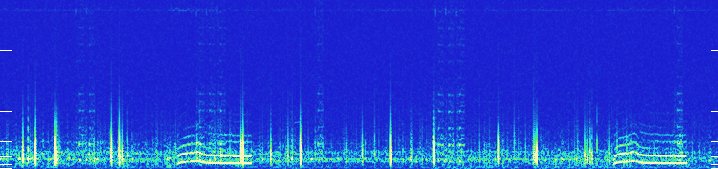
The picture
below shows a compressed time period of about two hours:
Signal type 1a:
Noise
"pulses"
In some cases, the noise periods of this
pattern
contain sinusoidal components, modulated in their frequency and
looking
like a kind of Information. The following example shows weak
signals of
the same structure during the absence of the strong signal,
looking like
a data transfer between a near and a distant station (signal
type 1b).
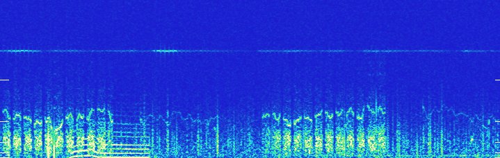
Signal type 1b:
Noise
"pulses" with sinusoidal components (including a signal of
type 2 in the
left part).
The straight line at the upper part of the
picture
is the 16 Hz signal of the railway power lines.
Signal
Type
2
A signal pattern which appears day and night
at
irregular time intervals. The signal contains many harmonics and
lasts
several minutes. The waveform and the frequency is changing
during the
presence of the signals. All received signals of this type are
identical,
no matter what time, day or year it is. There seem to be two
independent
sources, sometimes interfering with each other. One source is a
little
bit lower in its frequency than the other one. Played back at
160 times
the original speed it sounds very strange like a human voice
saying “Helloooo”
very slowly.
Signal
Type
3
Almost permanently, there are additional,
short
signals of constant frequency with a great number of harmonics.
Usually,
they are grouped together in two to three units and sound like
geese, when
played back at 160-times speed.
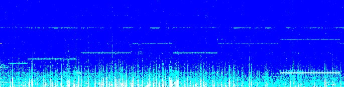
Signal Type 2 and
3
recorded at the same time (time range showing approximately 1
hour of recording
time)
Signal
Type
4
This category of signals does not appear so
often
and consists of a sequence of constant sine waves, jumping to a
higher
frequency after a constant period of time. In the spectrum
versus time
analysis, it looks like a stair. Played back 160 times the
original speed,
it sounds like someone is playing a flute. These signals are
also completely
identical across the many months I received them.
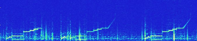
The picture shows
three
signals of type 4, recorded at three different days for
comparison
Signal
Type
5
At irregular time intervalls, a very strong
noise
signal with no specific structure can be detected. This noise
sometimes
lasts several days. The amplitude of this noise is about 10 or
even more
times stronger than the amplitude of the signals described
above.
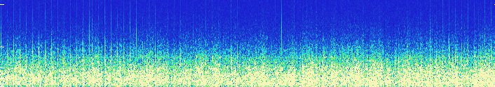
Strong noise
signal
of type 5
Signal
Type
6
Beside the known 16.66 Hz sine wave signal
caused
by the power for electric trains, sometimes strong sine wave
signals appear
at lower, different frequencys which sometimes are interrupted
and sometimes
suddenly switch to different frequency levels. Played back at
160 times
the original speed, it sometimes sounds like a radio teletype
communication
on shortwave.
Constant sine wave
signals of different frequencys.
The strong line at the lower right part of the picture is a signal of 5 Hz which was repeated very often in the last weeks before this page was written
Another strange discovery
After a while I discovered, that the signals got stronger, when the coil antenna was directed towards the ground or even laid flat on the ground. This brought me to the idea, that the signals might come directly from the ground or even were produced by currents in the ground. To find out more, I replaced the coil antenna by two metal sticks as probes (long srew drivers), put them directly into the ground (a meadow behind the garden) with a distance of approximately 4 meters and connected them to the amplifier.
The result was fascinating: The same signals I received by coil now reached the receiver via the two probes. Could it be that I had done some mistake?
I took one probe (the mass potential) out of the ground. If the signals had come from electric fields in the air, they would have been present now, too. But they disappeared. Only when the two probes were in good connection with the ground, the signals appeared. This proved that there was an electric current flowing through the ground – strong enough to create proportional magnetic fields that could be detected by a coil. Interesting to me was also the fact, that these currents obviously seemed to flow directly in the upper surface region of the earth. From this moment, I continued my measurings by using the probes. There was a clear advantage: No passing cars or neighbours with metal tools or lawn mowers could spoil my measuring results any longer.
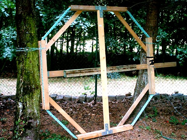
Coil Antenna with
400
turns, a diameter of 175 centimeters and a higher sensitivity
than the
discribed one
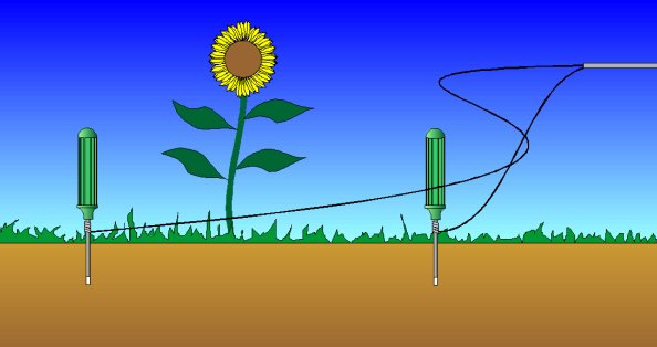
Using probes
(screw
drivers) instead of coils
Comments and common notes
All these signals were not only received in the area of my home, but also in two additional regions within Germany at a distance of several hundred kilometers. At all measuring locations, the signals were identical. Today (October 2003) the signals have been received for nearly three years at irregular time intervals of a few days.
No time pattern (rhythm of day and night, week and weekend or winter and summer) has been identified until now. Due to the implemented low pass filter, interference or modulation of higher frequencies can be excluded.
By reducing the filter intensity for testing purposes, the 50 Hz signal can also be made visible on screen. The shape of the 50 Hz signal proves that the above mentioned signals can not be a modulation of the 50 Hz signal: The 50 Hz signal is “riding” on the lower frequency signals. This shows, that it is not a modulation but a superposition, which only can be possible if there are different, independent sources.
The measurings were made in quiet agricultural regions. The chance that there are any industrial machines creating the signals is very low.
The signals are not only very low in their frequency, but also in their amplitude: The voltages at the coil and at the two earth probes are in the range of microvolts. As they are permanently covered by the relatively strong 50 Hz signal, discovering them is only possible with a powerful 50 Hz low-pass filter and a high-gain amplifier. May be that's the reason why these signals seem to be unknown to most of the people until now.
A different method often applied by other researchers is leading the signals from the probes or coil directly to the sound card of a PC and then analyzing it. The 50 Hz hum then is reduced to a horizontal line on screen. But with this method, only relatively strong signals can be detected. If you try to amplify the signals coming from the coil or the probes without a filter, the amplifier stage would be overdriven by the 50 Hz hum and clip the signal.
Function-Description of the ELF-Receiver-Amplifier
The circuit principly consists of three
different
stages, which form a unit, that can be repeated several times
until the
desired amplification factor is reached.
 |
These stages are: amplifier,
highpass filter
(DC-Offset suppressing) and low-pass filter (hum
suppressing). So, the
circuit diagram may be understood only as an example,
that can be modified
in the sense of the user, specially in regard to the
values of the resistors.
The first operational amplifier at the upper left corner of the diagram serves as an input stage with a low input impedance and an amplification factor of 180. The input can directly be connected to a coil antenna or (as open input) to the two earth probes described in the corresponding web article. |
The resistor of R3 (1k) between the non-inverting input of the operational amplifier and mass is necessary for common mode rejection. Without it, switching actions within a PC connected to the circuit could result in spikes at the signal.
The second Op-Amp A2 has a function as a high-impedance buffer for the CR-unit C1, R4 which forms the first high-pass filter stage. The cutoff frequency is lower than 1 Hz. The highpass-filters are absolutely necessary: Due to the high amplification of the whole circuit, the low DC-Offsets of the single amplifier stages would multiply and would result in driving the whole system to its clipping range ( minus or plus15 V).
After the first high-pass, the first low-pass filter is following (R5, C2). A3 serves as buffer for that low pass. The low-passes are attenuating frequencys in “higher” ranges (near 50 Hz). If they would not be implemented, the 50 Hz hum present nearly everywhere would result in driving the whole system to its clipping range: Nothing but a 50 Hz rectangular wave would be seen on the screen of the scope.
With A4, A5 and A6, the whole “procedure” repeats itself: A second unit, consisting of another amplifier, a high-pass and a low-pass filter is following. The third amplifier stage, realized by A7, is adjustable in its gain by P1.
Turning P1 to zero, a gain of 12 will be achieved (related to A7). Turning P1 to maximum, the gain of A7 is about 1.5. A7 also serves as a mixer for the offset adjusting voltage. This voltage adds an offset to the output signal. This will be necessary, if the amplifier is connected to an A/D-converter which only accepts positive input voltage.
The gain of the offset voltage at the output of A7 is equal to R11/R13. This means: the ofset Voltage is not amplified (R11 / R13 = 1) and easily adjustable by P2 between 0 and +5 Volts. Don’t forget that all amplifiers in this circuit work as inverters. That’s the reason why the voltage at P2 must be negative to achieve a positive offset voltage. The negative stabilizer 7905 is very important: Without it, the zero-line of the displayed signal could shift, if the supply voltage changes in case of battery supply. If you supply the circuit by battery, you may ommit the stabilizers 7815 and 7915, but not the stabilizer 7905.
If you only find a 7805 instead of a 7905 in
your
spare part shelf, you can add another inverting amplifier
between A7 and
A8 to turn the negative offset into a positive one. The values
of the resistors
(between the inverting input and the output respectively between
the output
of A7 and the inverting input of the additional amplifier) in
this case
must be equal: for example 180 k.
R12 and C5 build up a last (safety) low-pass
filter
together with A8, before the signal is carried to the output. If
you like,
you also can add another stage consisting of amplifier,
high-pass and low
pass instead of the single low-pass shown in the diagram. But
remember:
With each amplifier stage, unavoidable noise disturbances will
grow, which
often may not be distinguishable from a received signal.
Power
supply
The power supply creates a stabilized voltage
of
two times 15 Volts symmetrical, realized by a transformer with
two independent
secondary 15 V coils. With two independent secondary coils, you
also can
build up two identical positive supply stages and then connect
the negative
output of the first supply stage to the positive output of the
second one.
This connection then corresponds to the common mass at the
circuit shown
here. If you use the power supply circuit shown in the diagram,
you can
also use a 15 V double transformer with only one secondary
middle connector.
The power consumption of the circuit is very low, so the
stabilizers do
not need any heatsink.
Testing
the
circuit
Before using the circuit, connect the coil to
the
input and put Op-Amp A1 into its socket. Then check its output
signal with
an oscilloscope (Switch to DC-Input). The output signal must be
a DC voltage
which should not be bigger than a few hundred millivolts in the
positive
or negative range (“natural” offset of the Op-Amp). Put A2, A3
and A4 in
their sockets.
Then check the output voltage of A4. The
result
must be equal, but if you use a strong magnet and move it by
hand and near
to the coil, a corresponding signal must be detectable at the
screen of
the scope. If not, check the outputs of A2 and A3: If the
voltage is in
the range of some volts, something is wrong. Check the wiring
and use different
Op-Amps.
After the next amplifier stage (A7), you can
keep
a bigger distance to the coil to reach the same result described
above
with the scope. Also, any 50 Hz hum must be getting weaker after
each filter.
When checking the last stage (Output A8), a normal sized loudspeaker magnet still must create sinusoidal waves at the scope at a distance of approximately 10 meters if it is moved by hand. If the amplification still is not strong enough, see last section of this paragraph.
To finish checking, turn the variable resistor P2: A changing of the DC-offset must be visible at the oscilloscope (Don’t forget to switch the scope input to DC).
If no magnet or metal piece is moved near the
coil,
only an extremely weak ground noise should be seen on the
oscilloscope.
If you have a strong noise in spite of this, maybe you should
change one
of the Op-Amps: something must be wrong.
Be sure to use no wrapped capacitors. They may
pick up radio frequencys.
It is not possible to give a definite information about the total gain of the receiver as this depends on what signals you are receiving and how strong the signals of your interest are in your region.
Normally, the receiver works well if the test with the magnet is OK and if there ist no additional disturbing noise created by the amplifiers.
If you watch the output signal of the receiver for a while and then suddenly you may detect some unusual signals, you can try to amplify them a little bit more by reducing the values of the resistor R10 down to 4,7 k. If this won’t be enough, you can raise the values of R7 and R11 from 180 k up to 470 k or even 1M.
Remeber: The gain of an inverting amplifier stage is R11/R10 (if we look for example at A7). So you have to double R11 or to take half of R10 to double the amplification of the signal that’s coming from the output of A6. If you do both, the amplification will be 4 times as high as before.
Filter
transfer
function
Only at a frequency of 1 Hz, the amplification
corresponds to the values which can be calculated by the
resistors of the
amplifier stages. For higher frequencys, the amplification
constantly abates
and reaches an extremely small value at 50 Hz, which is suitable
for hum
suppressing.
Conclusion
Finally the question remains, who on earth is practising communication via such low-frequency signals and additionaly “abuses” the earth as a kind of wire? The structure of the signals leads us to the assumption that they are man-made and not of natural origin. But officially, military communication between submarines is in a range about 70 to 80 Hz. So where do they come from, these signals? Maybe further investigation will show.
Technical notes
All diagrams are spectrum versus time analyses.
The maximum amplitude range in the corresponding time signals of all diagrams is zero to plus 0.6 Volts (after an amplification by the factor 240000).
The displayed diagrams show a receiving time between approximately 1/2 to 2 hours.
The sampling rate in all diagrams was 50 Hz.
About the author
The author of this web page, born in 1948, is
geologist
and lives in Germany.
Author web page: http://www.subroutine.jimdo.com
For references and contact see to the
collaborators
list: http://www.vlf.it/directcontact/directcontact.htm
Thanks to Joerg Benscheidt, a translator and writer who helped me creating the final English version of this article.