This article describes an experience of radio seismic emissions monitoring, that is those radio signals emitted during the earthquakes. The sensors used (orthogonal earth dipoles) and the analysis used on data (the directional spectrogram) makes the difference from all other monitoring studies done so far.
PRECEDING RADIO SEISMIC EXPERIENCES
When, some years ago, I started the research on
radio seismic experiences I was very enthusiastic. On magazines and internet
It was possible to read about the possibility of forecasting earthquakes
with the help of earthquake radio emissions. It is not very
difficult find documents about noise covering the entire radio spectrum,
about TV emissions disturbed a few hours before an earthquake, about scientists
who forecast an earthquake
but in all those cases two things was
missing:
- technical data qualifying the phenomenon (frequency,
intensity spectrum), and so consequentially:
- the repeatability of the acquired experiences
But the subject was simple: if the devices not projected for receiving these emissions, was disturbed by them during their functions, an observation more careful would have given better results.
I've done, so research at 360°. I studied all
seisms in a ray of 1500 km from my QHT (which is a seismic zone),
by using data coming from South Europe observatories, which are, fortunately,
very numerous. Since I didn't know exactly what to look for, I set up a
1/100 Hz monitoring system using both antennas electric and magnetic:
- a big T, 11m high with double top hat of 45m
- a big horizontal loop, 3 turn, 30m x 30m
- an earth dipole of 30m, NS oriented as by ELFRAD
prescriptions
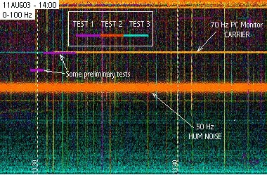
|
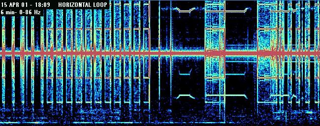
| This picture shows a 10 hours acquisition with a T Marconi antenna and spectrum Lab software in a 0-100 Hz range. The weak signals between 1 and 3 Hz created due by the antenna microphone effect, and are done by the wind which makes the wire structure move. |
All systems used were extremely sensible so that they could get even the natural background noise in that frequency range, such as Schumann resonaces, or the 82 Hz military emissions towards submarine immersions. The acquired data was possible by "auto saving pictures" feature contained in the spectrogram software used. In a year were saved about 3000 spectrograms and the gotten data were compared to those of 130 earthquakes of magnitude 2,5.
Results were, to me, puzzling: neither in local seismic episodes (where I could feel glass shacking inside the cupboard) nor in very distant events I could associate radio emissions to earthquakes. I exchanged experience with Prof. Ezio Mognaschi (see the article On the possible origin, propagation and detectability of ELECTROMAGNETIC PRECURSORS OF EARTHQUAKES), Vittorio De Tomasi, Dave Oxnard (ELFRAD) and con Wolfgang Büscher (SpectrumLab Author). The choice of the setup (frequency range, spectrum resolution, time scroll ...) is my personal synthesis of collected opinions and suggestions.
What follows is a personal contribute of their and our experiences.
FREQUENCY AND PROBES
The choice of the utilized sensors, as in ELFRAD
research, in based on earth dipoles.
I like the idea of using the earth as a big human
body and to consider stakes in the ground as sensors on skin. If those
emissions, caused by the rock ruptures, exist, it may be easier to detect
local currents directly instead of detecting the electromagnetic waves
which are generated by these currents. Since the length wave are from 3000
to 3000.000 km we are 99% in the near field and not in the one radiated.
Given up the old reception system (the big loop
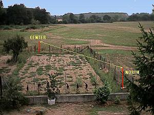
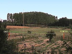
and big Marconi antenna ), three stakes are put in the ground. The
first goes as center, the second as vertex (respect the first), and
the last at east. Two dipoles (center-north and center-east) are 25m one
from the other and 50 meters from the house (and so 50 m from electric
lines). Stakes resistance changes from the season to season, and it changes
even according to the ground humidity, set normally about several hundreds
ohm.
 .
. 
After trials done on signals truly radiated (as the ones of submarines versus at 82 Hz), the earth dipole is not much sensible under 1000 Hz. With earth dipoles it is not possible to receive Schumann resonaces (7, 14, 21 Hz) which are anyway present with strong intensity (about 10 pTesla). Comparing spectrogram done with vertical antennas and earth dipoles, we can easily see that many statics are not receivable in lower frequencies with earth dipoles, when at the same time the low frequency spectrum is strong and clear with electric field reception (as with big T antenna); earth dipole is still a perfect whistler and tweaks receiver, under 1 khz is less strong in sensibility, for electric vertical signals.
But with earth dipoles we can receive lots of signals under 150 Hz. What are they, so?
The answer comes from comparative trials of signals
acquired with earth dipoles and the ones with big horizontal loop (loop
30X30m).
Basically the spectrograms under 150 Hz are equal.
Maybe that's because received signals are not irradiated but created by
ground currents: do not forget that in a nation little as Italy a power
of 50000000000w (50.000 MW !) is used, and big quantity of electric spurious
are injected in the earth by ground connections. An earth dipole may even
work as a 'skin' sensor, catching the current flowing in upper ground levels
- like a simple tester measuring the resistance.
The big horizontal loop takes the same signals since in such low frequencies doesn't only work as antenna but also a transformer: vacant currents go through the earth surface creating a magnetic field and a loop tension.
These currents don't have linear paths, since their
path is conditioned by the ground resistance, which changes from
season to season and from place to place. The same signal source
can so be gotten from different directions at a certain distance after
a big rain.
The radio localization of these signals so gets
a very doubtful aspect. Since the path is not necessarily a straight line,
it is almost impossible to presume the source of the signal only by observing
the angle of arrival.
Why, so to set two orthogonal antennas? They
are difficult to place correctly, they request lot of space and the results
do not give the direction data.
The choice of having two dipoles, instead of only
one (as ELFRAD setup) gives two benefits: first no receiving null (as for
the currents which go perpendicular to the dipole direction) the second
to add a data to arrival signals: the color which identifies the direction
of arrival can ease the detection of a very weak signal or noise hiss coming
from a different direction, though the signal is below the noise floor.
So we are able to find signals even if a simple single FFT gives noise
only.
FREQUENCY
Another big question is which frequency range which
must be monitored, and which can be monitored without a lot of annoying
noise.
The literature available in "do by yourself" experiences
(not documented by scientific protocol) nearly goes to science fiction:
we can find references about seismic precursors which go from DC to many
GHz, and energy emission gotten only by "sensitive man" or cats, or better
written many years ago in the Nostradamus triplets... the landscape is
very colored!
Here, we stop at experimental tests of Us
Geological Survey Calculations (905A National Center, Reston, VA 20192
USA) which indicate in a broad frequency range (0.1 to 50 Hz), a good observation
points for all events. The target of this experience is not to find seismic
precursors but to determinate if there is or not emission of receivable
radio frequency during the earthquake.
There is now a new problem: how to distinguish
a main power noise or an experimental mil transmission from a seismic precursor?
The gotten signals arrive to the earth dipole by
the same way both if they come from the underground and if they come from
an electric station or from a steelworks far 25 km away: that is current
going in the ground.
To avoid this problem the frequency covered by our monitoring goes up to 125 Hz: noises coming from electric ground connections are often mirrored to main power frequency. If you receive a pulse tone at 10 Hz by observing at 90 Hz you got the same tone (and sometimes even 110 Hz). These signals very well known to those who observe with earth dipoles very common receivable both in America and Europe would seem caused by high power electric energy regulation devices.
At example: the steelworks' oven controls the fusion
temperature pulsing the current (we are speaking of many MegaWatts power):
a pulse current (on/off type) at 30 Hz on a three phase system, modules
in AM the 50 Hz carrier (or 60Hz in US), generating two side bands at 50+30Hz
and 50-30Hz, then at 20Hz and 80Hz.
The 98% of the receivable signals with earth dipoles
has there characteristics: are specula with electric frequency. It is clear
that such a signal nothing has to do with radio seismic signals and with
military emissions.
AUDIO CARD INTERFACING
No special acquisition hardware was required for these experiments, only a normal PC audio card. Some components are used to interface the dipoles with the line input of the Sound Blaster. The acquired signals must be totally floating, or in other words be insulated from the audio card's ground. If you connect the ground pin of your audio card with the "CENTER" stake of the antenna, there would be an unwanted short circuit from your PC towards the earth antenna, distorting the signal with a lot hum noise, and making the RDF functions useless.
Earts dipoles are connected to two toroidal transformer
for power supply 12v/220v 10w: the antenna is directly connected to the
high voltage winding with a 10 kOhm resistance in parallel, and outputs
comes from the low voltage winding; 10 kOms resistance utilizing allows
the extension of the frequency response of all system up to 20 KHz, if
you want to utilize orthogonal dipoles in order to receive whistlers, tweaks
or RTTY emissions.
The signal output, is then pre amplified by a OP07
operational amplifier, set up as described in the article of Ik1odo The
use of low noise OP AMP" on this web site. The system so set up went
all right for 10 storms with no damages for preamplifier, nor audio card.
But, despite the antenna is DC isolated from the
rest of the station, is useful to cut the connection to earth dipoles when
there is a storm.
TYPE OF ANALYSIS: DIRECTIONAL SPECTROGRAM
There are different opinions about that, which representation
can indicate at the best the presence of radio seismic signals.
Starting from the analysis based on the time, on
the medium spectrum for a certain gap time, up to waterfall display spectrogram.
WinQuake software, utilized by Elfrad research
project, for instance gives more attention to an accurate study to signals
which change in amplitude versus time. Custom card for acquisition records
in fact starting from DC to 25 Hz and the software gives graphic representations
of the gotten signal with many types of filters and sensitivity.
In this particular case, a special type of spectrogram
was chosen: a dual-channel, complex FFT, which produces a directional spectrogram.
I think this is the type of analysis which can
detect the presence or the variation of minimum quantities of noise or
of the signal a bit better than the traditional spectrogram. Even
broadband noise can come from a certain direction!
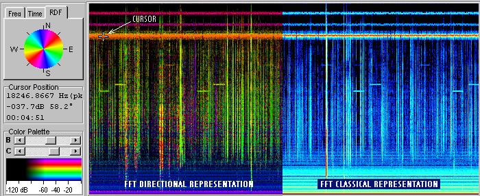
While in a traditional spectrogram with a color palette, or monochrome one, different colors are associated with different signal intensities; in a directional spectrogram the color (hue, or "tone") indicates the main direction of the signal while the brightness is an indicator for the signal strength. We handle a very complex type of representation and at the same time, more information on the screen (which shows frequency, time, amplitude, and angle information simultaneously).
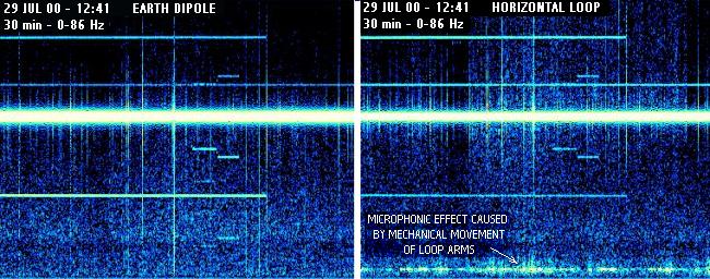
The following picture shows the difference
between a simple spectrogram (the right side elaborated by Richard
Horne palette) and a directional one (the left part with FFT complex and
the different color palette).
The cursor position on a signal gives instantly
the provenience direction, frequency and level. The reception
of the pictures below has been done with earth dipoles.
The Color Direction Finder
in Spectrum Lab is based on a DOS QuickBasic-program written by Markus
Vester, DF6NM. He made an excellent paper about the principle and some
applications of his program (which btw is more versatile than the Color
Direction Finder implementation in SpecLab).
It is a special kind of Spectrogram
("waterfall") which shows not only the intensity of a signal, but also
the azimuth angle. The azimuth ("compass direction") defines the color
tone, the intensity (total field strength) affects the luminosity. The
bearing (azimuth) is calculated only from the voltage ratios and the "polarity"
(0° / 180°).
The program only sees the
phase difference (here: sign) between the two antennas but cannot detect
the absolute phase. If there is 0.707 V from the N/S and 0.707 V from the
E/W loop with 0° phase shift between them, the transmitter may be in
the northeast or in the southwest (only the more complex system "E-field
antenna and two combined loops" can solve this ambiguity, because the E-field
antenna is used like a phase reference there). Here, only a 180° compass
range can be displayed.
Spectrum lab of Wolfgang Buscher DL4YHF can be directly downloaded at http://www.qsl.net/dl4yhf.
WORKING PRINCIPLE
IN ORTHOGONAL ANTENNAS
(How two fixed
identical antennas can find the direction of a signal)
The signals from two orthogonal antennas are fed into the left and right audio input of the sound card. A special software calculates spectra ("FFT"s) from the nort/south and east/west antenna, which contain phases and amplitudes for a large number of different frequencies. The amplitude ratio and phase between the two inputs can be used to calculate the angle of arrival.
Ideally the phase between the two inputs is either
0° or 180°, but nothing else. The bearing (azimuth) is calculated
only from the voltage ratios and the "polarity" (0° / 180°). For
example, there may be a fictional transmitter inducing up to 1 mV in main
direction of any antenna. Let the fictional transmitter move around the
observer's location ... the antenna voltages will be:
| Signal from the north: | U_e/w = 0 mV | U_n/s = 1 mV | phase doesn't matter |
| Signal from the northeast: | U_e/w = 0.7mV | U_n/s = 0.7 mV | 0° phase difference |
| Signal from the east: | U_e/w = 1 mV | U_n/s = 0 mV | phase doesn't matter |
| Signal from the southeast: | U_e/w = 0.7mV | U_n/s = 0.7 mV | 180° phase difference |
| Signal from the south: | U_e/w = 0 mV | U_n/s = 1 mV | phase doesn't matter |
| Signal from the southwest: | U_e/w = 0.7mV | U_n/s = 0.7 mV | 0° phase difference |
| Signal from the west: | U_e/w = 1 mV | U_n/s = 0 mV | phase doesn't matter |
| Signal from the northwest: | U_e/w = 0.7mV | U_n/s = 0.7 mV | 180° phase difference |
Looking at this table, there is obviously a 180°
ambiguity for the simple "two-antenna" configuration. Why ?
Because the program can only see the phase difference
(here: ideally 0° or 180°) between the two antennas, but it can
not see the absolute phase of the voltages induced in each antenna. For
this reason, all possibly color values appear two times on the 360°
compass. (There is a solution for this ambiguity, but it requires
a more complex antenna setup and is not the subject of this article.)
As already mentioned, the software calculates amplitudes and directions not only for one single frequency, but for a large number of different frequencies. The results are displayed on the screen in a special kind of spectrogram, where the color indicates the direction and the intensity shows the signal strength.
AMBIGUITY OF GOTTEN SIGNALS
It's very important, though, to be clear about some
specific details when detecting the direction with the dual-channel FFT
and earth dipoles.
 |
The earth dipole is a very special antenna, even
the definition of antenna is strange for it and not suitable: while a vertical
rod receives the vertical electric component only, and with a loop the
magnetic one only, but for the earth dipole things are combined - it's
actually a mixture between the two previous antenna types.
In some situations the earth dipole acts as a vertical loop, put into the ground and oriented in the two dipole's direction. In this context it can be considered a directive antenna in B field. But if a horizontal electromagnetic field exists parallel the two dipoles, they work as an electric horizontal dipole, and even in this case, receive the incoming signal. And the same is true for earth current injected in the ground by electric ground connection. |
It is true that during the day, signals in the VLF spectrum have vertical electric polarisation, and travel via ground wave; but during the night reflections can be make the components rotate; which causes fading when received with an orthogonal loop system, but with earth dipoles we see a change in the signals prominent direction (apparently a non real thing).
If we add all of these non-irradiated signals, but
simply ground injected through earth connections and electric distribution,
and the free-flowing current from the earth magnetism effect, we have a
large view which takes us away from the original RDF concept. The following
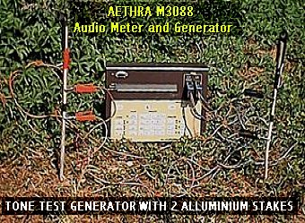
picture shows an example of ground injected current.
At a distance of hundred meters from the orthogonal
dipole system a 80 Hz current is injected by means of an audio generator.
The transmitting dipole was then oriented in three
different angles, but preserving the same distance from the receiving antenna:
Though the signal still came from the same direction, the RDF diagram correctly
shows three different directions of the received current. Picture in the
following paragraph shows layout of the dipoles' position on the ground.
 |
 |
Why, then the choice fell on this particular type of elaboration? Because in the variation of the received directions, or in the phase rotations of signals gotten from dipoles, there may be some conjunction rings with seismic phenomena. The compared analysis of variations of the noise under 25 Hz between a traditional spectrogram and a complex one, type RDF show very clearly that some variations are evident as color spots are not evident in a classical FFT analysis.
SYSTEM CALIBRATION
Even though, as already explained, our target is
not to determinate the exact provenience direction, but instead eventual
signal variations to the rule, it's anyway necessary to be careful in positioning
dipoles. A mountain climber compass, will give an orientation with precision
+ - 2°. It's useful to place the dipoles referring to the magnetic
pole and not to the geographic one. The correction due to magnetic declination
can be put in a software during the elaborating operation.
Particular attention must be given to the two amplifiers
calibration. Signals coming from the two dipoles won't show the same
intensity because of the ground irregularities. Two dipoles of the same
length, positioned few meter from each other , and with the same orientation,
have different resistance and consequentially a receiving reception different.
 |
We must so determinate the sensibility of every
single dipole. In order to do this we have to place a third dipole, center/north-east
oriented, that is 45° oriented: a dipole center calibration.
Giving a signal in this dipole we'll have a reception on other dipoles.
The preamplifiers will have to be regulated to have
the same reading from CENTER-NORTH and on CENTER-EAST dipole, using as
reference the readings on the audio card.
|
SPECTRUM LAB
For starting, getting and storing spectrograms
with SpectrumLab first we must to make some settings. Here you have a description
of the operations. This does not substitute the program instructions, which
have to be read before starting a complex RDF, but it's a simple track
to install a receiving station.
1 - Connect the "center-north" dipole only and verify
that on the spectrogram, in RDF mode, the images are blue color only (0°
or 180° direction)
2 - Connect the "center-est" dipole only and verify
that on the spectrogram, in RDF mode, the images are green-yellow.
If two things are inverted, switch the connection of two dipoles to the
audio card, or invert the settings in the "SpectrumLab Components
Window" (the SpectrumLab mixer).
3 - Once verified the correct channels connection
, we can give another trial signal in center test dipole. In our case we
inject a 10dBm signal at 80 Hz frequency. The visualized color must
be red (corresponding to 45°). If it's light blue (corresponding to
135°) this means that one of the dipoles has been inverted in polarity.
So, or you switch the output (or the input, is the same) on the transformer
or you invert the rotation sense by software, switching the "rotational
direction settings", cw (compass style) / cww (math. style).
Once these operations have been done the system
is ready to go.
SpectrumLab make automatically save both spectrograms
and original signals gotten in decimate sample wave. We just have to chose
the saving mode data.
Some trials have been done about system frequency
linearity, to determine if the RDF representation works correctly in all
the used audio spectrum. A 80 Hz dipole "center/calibration" signal has
been injected and a SpectrumLab reading at 45° reception corner has
been done. The same trial has been repeated at 2200 Hz and 18000 Hz.
The maximum error obtained was 1.2° only, that means that dipoles system
react in the same linear way on all audio spectrum.
This precision featured is not usable for RDF operations
on frequencies higher about RTTY signals, where, always for the ambiguity
before shown (mixed effect horizontal/vertical polarization), gotten directions
do not correspond always precisely to effective signals provenance and
direction.
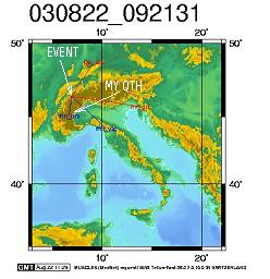
AN EVENT MONITORING EXAMPLE
During the first month of activity monitoring we
revealed some seismic events, which someone reveal from seismic nets
only and even some diffused from radio and television broadcast. Here you
have an example of a seismic event arrived at 150 Km far from my QHT in
Switzerland.
The event, magnitude 3.47 was even gotten from
the seismic observatory few kilometers from my home, part of MEDNET
network, from where these data were obtained, and from others three stations
in Switzerland, North-East italy and center Italy.
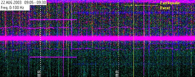
The directional spectrogram, further than usual
hum noise signals, is not related to the seismic event. The earthquake
is temporarily marked with a yellow vertical line to be recognized and
localized in the time scale. It seem there are no particular signals,
nor natural noise floor variation and nor in the direction of present signals,
indicating a radio emission associated to this seismic event.
CONCLUSIONS
The experimentation type offered can easily
be reproduced.
It is not necessary particular devices and
and the cost is really low: n.3 "one meter" copper tube (used as
stake in the ground), two toroidal transformer by power supply and a couple
of integrated circuits with few components around (no more than 30 $)
The gotten information, which contain data about
both dynamic and signals direction, is really remarkable.
Who knows if it's with this system that we'll
see for the first time the real radio image of an earthquake?
Many thanks
to:
Andrea Bertocchi for Italian to English translate
Marco Bruno and Wolfgang Büscher for technical
support an revise.