The project is called Listening Observatory. You can see it at https://listen.vrontier.org/ and the software is open source (link at the end). I should say at the start that I am not a VLF specialist. I came to this from the software side, out of curiosity about what a computer can notice when it listens to one place for a long time. I built it together with an AI assistant, Claude by Anthropic: it helped me analyse the recordings, write the software and draft this article; the choices, and any mistakes, are mine. So this article explains the method, in simple terms, and it is honest about what the method cannot do.

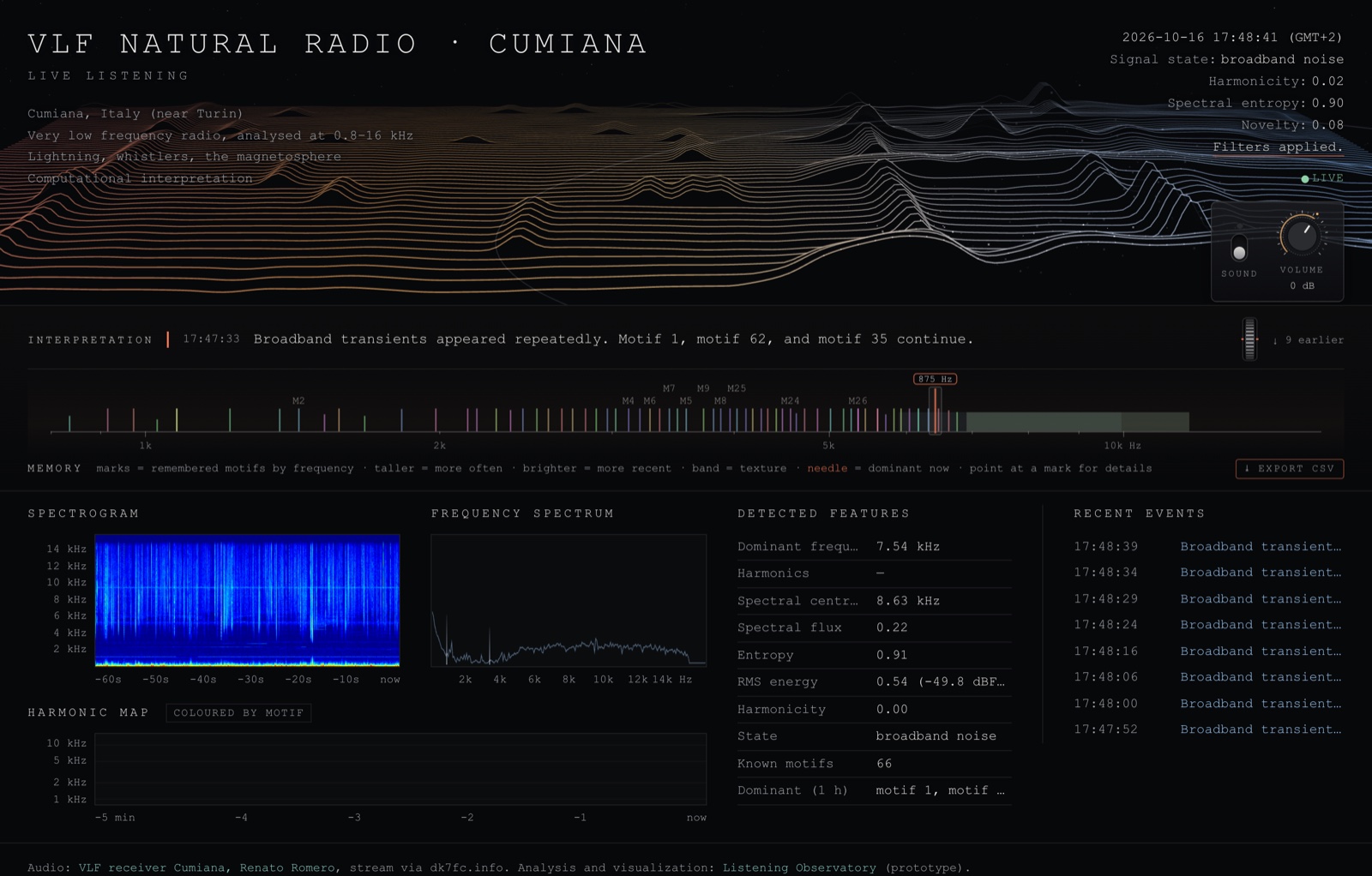
Fig. 1 - The live page for Cumiana: the landscape on top, the memory dial in the middle, the analysis panels below.

THE CHAIN
The system has four parts, one after the other:

1. A program on a server receives the stream and decodes it.
2. The same program analyses the sound: spectrum, peaks, sudden events, steady lines.
3. A memory compares what is heard now with what was heard before.
4. The browser of each visitor receives the results as small messages and draws them.

A fifth part, a language model, writes two short sentences about what was measured. It comes last here because it is the least important part for a radio listener.

One copy of the program runs for each stream. It is written in Go, and it uses the free tool ffmpeg for decoding. It needs very little: several streams run together on a small rented server.

VLF station audio stream on the Internet

→

Decoder ffmpeg 32000 samples/s

→

Analysis FFT, peaks, transients, lines

→

Memory motifs, 30 days of events

→

Browser messages in, pictures out

Fig. 2 - Block diagram: stream, decoder, analysis, memory, browser.

RECEIVING AND DECODING
The stream arrives over the Internet as compressed audio, exactly as a listener would receive it in a media player. ffmpeg decodes it and hands over plain samples: one channel, 32000 samples per second. As "FFT for dummies" explains, the highest frequency we can then represent is half the sample rate, here 16 kHz.

Streams break. A connection drops, a station restarts, a relay is busy. The program reconnects by itself, at first after one second, then waiting longer each time, up to five minutes. Time without signal is not counted as listening time, so an outage does not appear later as "silence".

THE SPECTRUM
The samples go through an FFT, in the usual way:

- FFT size: 4096 samples, which is 128 ms of signal
- frequency resolution: 32000 / 4096 = 7.8 Hz
- window: Hann
- a new spectrum every 50 ms, so 20 spectra per second (the windows overlap)

For Cumiana the analysis looks at 800 Hz to 16 kHz. This keeps it on the part of the band where sferics, tweeks, whistlers and chorus are heard, and away from the lowest frequencies, where most of the interference from the power grid lies. With 7.8 Hz resolution and this lower limit, the system is of no use for the ELF band: Schumann resonances and anything else below a few hundred Hz are outside its view.

Each spectrum is then reduced to bands, in two different ways. For the analysis and the landscape there are 48 bands, spaced logarithmically between 800 Hz and 16 kHz, each about 6% wide. For the spectrogram there are 240 bands of equal width from 0 to 16 kHz, each 67 Hz wide; every band takes the strongest frequency inside it, so a narrow line keeps its level. The spectrogram bands are not filtered: the harmonics of the mains stay visible there, because the filter only applies to the analysis. Both sets, ten times per second, are what the browser receives.

The levels are relative, not calibrated. The program follows the range between the quiet and the loud bands over about five minutes and scales the picture to it. This keeps a weak stream and a strong one equally readable, but it means that the display says nothing about field strength.

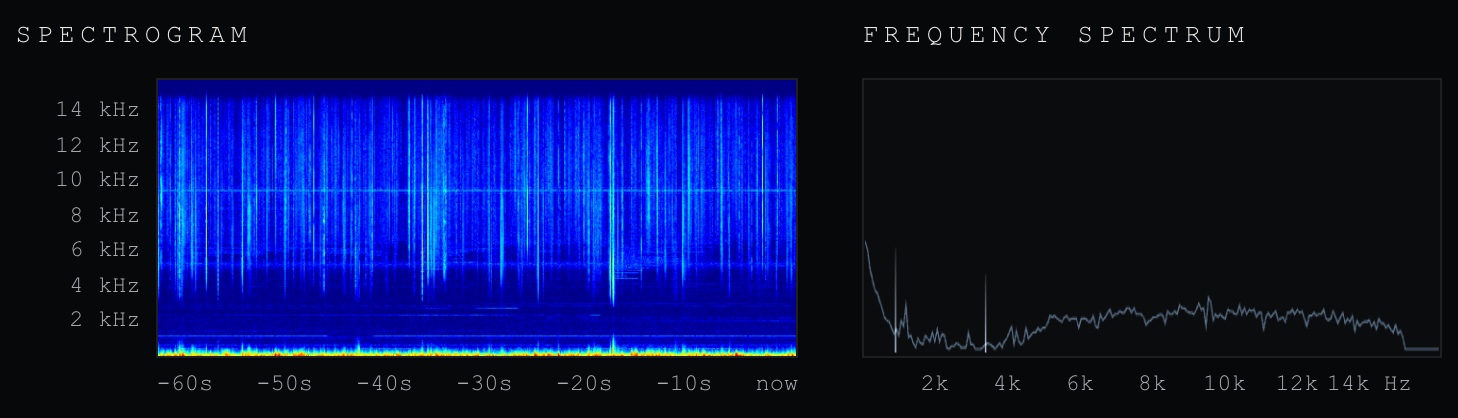
Fig. 3 - Spectrogram and spectrum panels for Cumiana, on a linear frequency axis from 0 to 16 kHz, in the colours of measurement tools: blue for weak, red for strong.

WHAT IS MEASURED
From every spectrum the program computes a few numbers. Each one answers a simple question.

- Level: how strong is the signal now, compared with the last minutes?
- Centroid: where is the "centre of gravity" of the spectrum, low or high?
- Entropy and flatness: is the energy spread over all frequencies, like noise, or concentrated in a few lines?
- Flux: how much did the spectrum rise since the previous one, 50 ms ago?
- Harmonicity: do the peaks fit a series f, 2f, 3f...?
- Novelty: how different is the sound from the last minute?

Peaks. A peak is a point of the spectrum that is at least 8 dB above the median of its neighbourhood, one sixth of an octave to each side. Up to twelve peaks are kept. Peaks that lie on a multiple of 50 Hz (within about 12 Hz) are thrown away as mains hum.

Transients. A transient is a sudden rise across a wide part of the spectrum. The program keeps the flux of the last three seconds, takes its median, and waits for a value far above it; in addition at least 30% of the bands must rise by 3 dB or more at the same moment. On a VLF stream the sferics crackle all the time, so for Cumiana the threshold is set higher than for other sources and at most one transient is reported every five seconds. What the page shows as a transient is therefore a strong burst that stands out from the normal crackle, and not every sferic.

Steady lines. A peak that stays at the same frequency for at least five seconds, is present in at least 60% of the spectra in that time, and stands on average 10 dB above its neighbourhood becomes what the software calls a "resonance". The word comes from the acoustic sources the project also listens to, and it is misleading for radio: it has nothing to do with Schumann resonances. On a VLF stream a "resonance" is simply a narrow line that holds: a transmitter, an interference, a harmonic of something nearby. If other steady lines sit at two to eight times its frequency, they are attached to it as its harmonics.

State. Twice per second the numbers are put together into one word that describes the moment: quiet, transient activity, stable resonance, broadband noise, evolving texture and a few more. The rules are fixed and simple. For example, low harmonicity with a high centroid and high entropy gives "broadband noise", which is what a field of sferics looks like to these measurements.

THE MEMORY
This is the part that differs most from a spectrum analyser. The program does not only show what is there now. It asks: have I heard this before?

Each steady line is compared with the lines already known. The frequency counts most: two lines are taken as the same when they are within about 1.5% of each other, and the pattern of harmonics refines the comparison. A line that comes back often enough (three times over at least two minutes, or twice with five minutes of presence in total) becomes a motif. It receives a number and keeps it. When a motif has been absent for three minutes and appears again, the program reports that it has "returned". Candidates that do not come back within an hour are forgotten.

The same is done for the sound as a whole. Every 20 seconds a coarse fingerprint is taken (16 bands plus some of the numbers above) and compared with earlier fingerprints. Recurring ones become texture motifs.

The memory is kept in plain files on the server, with the events of the last 30 days. No audio is stored, only the measurements.

An example. The observatory has listened to Cumiana since 2 October 2026, and on 11 October its memory holds 76 motifs. The one heard most often is a line at 1436 Hz, seen more than 2600 times for about four hours in total. Many of the others form a ladder: 2125, 2282, 2434 Hz, then 3115, 3267, 3419, 3576, 3710, 3878, 4030 Hz, always about 152 Hz apart. It is not on multiples of 50 Hz, so the mains filter lets it through. Renato Romero, who runs the station, thinks these lines most likely come from the control systems of photovoltaic installations, which today send all kinds of signals through the power grid. A line that appears now and then at 1024 Hz comes from the Swiss power grid, which uses it to switch electricity meters between tariffs. Either way, these lines are man-made and not natural radio. This shows both what the memory is good at and where it needs a person who knows the station: it found a structure and followed it for nine days, but it took the station's operator to say what it probably is.

Fig. 4 - The memory dial for Cumiana: each mark is a motif at its frequency. Taller marks were heard more often, brighter ones more recently.

FROM THE SERVER TO THE SCREEN
The browser does not receive audio for the pictures. It receives small text messages over a permanent connection (a WebSocket):

- 10 times per second: the level, both sets of bands and the current peaks
- 2 times per second: the measured numbers and the state
- when they happen: transients, lines that start and end, motifs detected or returned

All drawing is done in the visitor's browser. The page has these parts:

- Spectrogram: one column per message, so ten columns per second. The panel is 600 points wide and shows the last 60 seconds, with a linear frequency axis from 0 to 16 kHz and the colours used by spectrum analysers and in research papers.
- Spectrum: the spectrogram's bands as a curve, and the peaks found by the analysis as bright needles.
- Harmonic map: the steady lines of the last five minutes with their harmonics, coloured by motif.
- Landscape: the same spectra drawn as terrain. Low frequencies are on the left, high ones on the right; height is level; the rows go back into the past. Steady lines rise from it as spires, and a transient sends a wave through it.
- Memory dial: every motif as a station on a radio dial.
- Tables: the measured numbers and the latest events.

The landscape is the artistic part of the project. It contains no information that is not also in the panels below it. It is there because it makes people stop and listen.

For Cumiana the audio can also be played on the page. The server relays the same audio that it analyses, and every message carries its position in that audio. The browser shows each event at the moment you hear it, so a crackle in the loudspeaker and the wave in the picture arrive together.

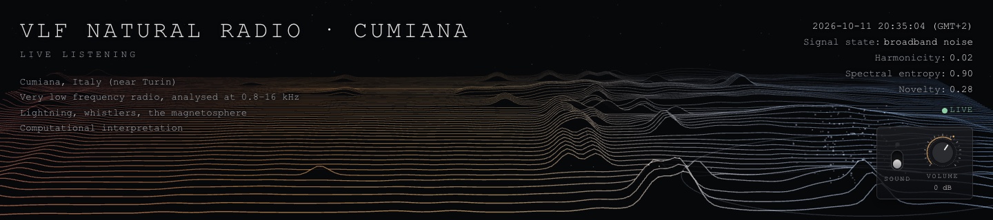
Fig. 5 - The landscape just after a broadband transient: the wave runs through the terrain at the lower right.

THE WRITTEN LINE
Above the dial there is a line of text, for example: "Motif 7 returned. Broadband transients occur while motif 83 and motif 23 continue." It is written by a language model, at most every 90 seconds, and only while somebody has the page open and something has changed.

The model does not listen to anything. The program gives it a short list of facts taken from the measurements, and the model only puts them into two sentences. Afterwards the text is checked: if it names a frequency or a motif that was not in the list, it is requested once more and then discarded. So the text can be clumsy, but it cannot invent a signal.

LIMITS
A VLF listener should know what this system does not give:

- The spectrogram is coarse: 240 bands of 67 Hz and 60 seconds. It shows sferics, steady lines and the general shape of the band, but it is not a replacement for SpectrumLab. A whistler lasts a second or two and covers only ten to twenty columns.
- Nothing below 800 Hz is analysed. The spectrogram shows that range, but the measurements, lines and motifs do not include it.
- The levels are relative.
- The stream is compressed audio, with whatever the compression does to weak signals.
- The software cannot tell natural signals from man-made ones. It finds what is steady and what recurs. Saying what it is remains a job for the person at the station.

CONCLUSIONS
A stream that is on-line can be more than something to listen to. With free tools and a small server, a program can watch it around the clock, keep a record of what recurs, and show the result to anybody with a browser. For natural radio the most useful part is the plain spectrogram, and that is where this project has the most to improve. Following Renato's suggestions it now uses a linear frequency axis from 0 Hz and the colours of measurement tools. The memory is the more unusual part: it gives a station a history that can be read back, of lines that come and go and of sounds that return.

Everything described here can be repeated. The software is free, and it works with any stream or recording you are allowed to use.

THANKS TO
Renato Romero, for the Cumiana stream, for the permission to use it, and for the suggestion to write this article. Stefan Schäfer (DK7FC), whose server relays the stream.

LINKS
- Listening Observatory: https://listen.vrontier.org/
- Source code (MIT licence): https://github.com/vrontier/listen
- R. Romero, "Create your own streaming VLF Audio program": http://www.vlf.it/obs3/mp3stream.html
- R. Romero, "FFT for dummies": http://www.vlf.it/fft_beginners/fft_beginners.html
- ffmpeg: https://ffmpeg.org/