 |
Of
all the bands where you can search for "Radio
Nature", the place of honor goes to the very
low frequencies below 100 Hz.
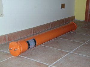
And the magnetic component of these signals certainly is the most interesting part: here we can find signals directed to submarines, Schumann resonances, geomagnetic pulsations caused by solar storms and, perhaps, the seismic radio precursors. An induction coil, also called search coil, is the prohibited dream for every "Radio Nature" researcher. They are available in commercial versions but the costs are very high: many thousands of Euros / Dollars for the coil and special receiving device. Let's see together how to build one with professional features for use with our sound card, but, spending far less money. |
A "BAD DEVICE", DIFFICULT TO MANAGE
The induction coil is nothing more than a multiturn loop and works with the same principle: there are many turns, a variable magnetic field passes through them, this creates a voltage across its terminals. In some loops we have no magnetic core and only mechanical support. Here we have a core material with high permeability, which virtually increases the efficiency and response of the loop/coils.
The reasoning appears simple, however, if we attempt to calculate this type of sensor we realize that it is almost impossible. Even the texts of physics and research institutes indicate that an induction coil is almost impossible to model. Fortunately we can resort to experimental tests to arrive at excellent results. Why? The reason is: there are too many unknown, unsuspected, and interactive parameters.
The first parameter that is difficult to calculate is the coil inductance. Even without considering the presence of a high permeability core, multilayer coils with thousand of turns are difficult to calculate. The final value of the inductor always has a different value from those calculated.
The second unknown is the parasitic capacitance: it changes its value depending on how the coils are wound, with what order, with how many layers. Two induction coils with the same look, same number of turns may have very different parasitic capacitance values: it involves two different values of self resonance, for example: 500 Hz and 4500 Hz... for two quasi-identical coils!
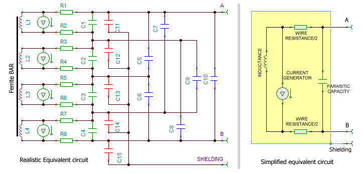
The third unknown factor is the
representation of an equivalent circuit. With an
air core loop, we can, with good approximation, reducing
everything to some equivalent components: inductance,
current generator, resistance and capacity. In an
induction coil we have the capacity between the
windings, capacitance between the layers, the capacity
between the sections, distributed resistance and mutual
induction is not constant between all of these. The
model presented in the picture does not accurately
simulate the approximate behavior of the induction coil
as it should.
 |
The fourth and most serious unknown
factor is the magnetic permeability of the system: we
have to use a core with permeability much higher that
the air to increase the effective capture area.
However, full effect of the high value of the
permiability is only realised with a closed magnetic
circuit, as in a toroid. In an induction coil the
core is open, which means that the effect is very small
if compared to original permeability and there are
considering the losses.
If we use a ferrite rod with a
relative permeability of 1000 we will not have an
increase of the capturing area and the inductance of
1000: the final value will be much lower and will depend
on the permeability of the bar used, the length and
diameter of the same. These two values are called
"rod permeability" (or µ rod) and "coil permeability" (µ
Coil) and, as if that were not enough, are not
equal! Here is an example with real numbers: one
induction coil with a core with µr of 500 (taken from
the ferrite data sheet) could have a µ-rod of 70
(inductance increasing) and a µ-coil of 30 (capture area
increasing). There are formulas to calculate these
values, but also they are only approximate.
Now you understand now why an induction coil is a difficult product to design? And perhaps this is the reason why they are so expensive.
THE CHOICE OF THE CORE: TYPE OF MATERIAL AND SIZE
The best results are obtained with
high permeability cores. The best choice would be
mu-metal or permalloy. But they are very expensive and
difficult to find. We therefore opted for ferrite: there
are many types and sizes, so there are many choices.
Also the choice of the length/diameter ratio is very
important: it must be as high as possible because the
rod-µ and µ-coils are heavily dependent by this value.
For ferrites like the one we chose, it must be at least
25 for a good coil efficiency. The numbers and the
choices that follow are the result of calculations and
measurements made on different materials.
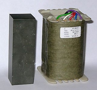 |
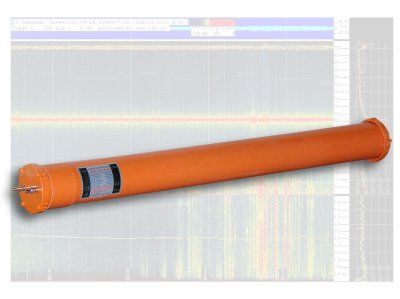
They are a good compromise
for an efficient coil and not too
expensive. We have chosen to use the rectangular
section ferrites used in power transformers,
composing a bar with the assembly of several
pieces. The material chosen was the code
I93/28/30 3C90 by FERROXCUBE: the value of µi
for this product at low frequencies is about
2300. They are high permeability blocks of size
3 x 2,8 x 9,3 cm. The core of the coil is
composed of 10 blocks and its final size is then
93 cm in length with a square section of 3 x 2,8
cm. The length / section is therefore
approximately 29 times, big enough to give a
good capture area.
In the left picture see a single ferrite block and a test coil. |
The final results, following the instructions that will be provided for the coil, are as follows: µ-Rod (ferrite reception gain) 158 times, and µ-Coil (ferrite inductance increasing) 71 times greater. These measured values indicate how large a change in the coil performance is achieved by adding the ferrite core. Both parameters are important: the µ-Rod will be useful to estimate the number of turns and µ-Coil to know the impedance and therefore properly design the preamplifier.
THE WINDING
With these data we are now able to determine the number of turns, referring to the formula to calculate the voltage at the terminals of a loop, immersed in a known field:
E[v] = (4 x 3,14 x N x A x 6,28 x F x H) / 10.000.000
- N is the numbers of turns in the loop
- A is the area of the loop in square meters, multiplied for the µ-coil value
- F is the frequency in Hz
- H is the magnetic field in Amps/metre ( B[µT] x 0,796)
http://www.vlf.it/minimal/minimal.htm
http://www.vlf.it/octoloop/rlt-n4ywk.htm
http://www.vlf.it/looptheo7/looptheo7.htm
The coil must be sensitive enough to receive signals such as magnetic pulsations and the Schumann resonances with an intensity much greater than its intrinsic thermal noise, and the noise that will enter the preamplifier front-end. We refer in this case the natural background signal levels indicated by Maxell and Stone in their treatise of 1963, which were as follows:
200 nT
@ 1 mHz
2,5 nT
@ 10 mHz
30 pT
@ 100 mHz
1
pT @ 1 Hz
0,3 pT
@ 10 Hz
0,1 pT @ 100
Hz
0,02 pT
@ 1 kHz
As a reference for the intrinsic thermal noise we have used the simplified formula:
Noise floor [nV/ sqrt Hz] = 4 x sqrt R [kohm] (sqrt stands for "square root")
We here omit the calculations and tests that led us to the final result: it was a long push and pull between calculations and experimental tests. Let's go straight to the final results. The coil will be built as follows:
- Number of turns: 96000
- Wire diameter: 0,16 mm (AWG34)
- Winding length: 80 cm
- Thick winding: 0,178 cm
- Length of wire: 13,44 km
- Weight of copper wire approximately: 2,5 kg
- Single turn area: 0,001225 square meters (3,5 x 3,5 cm)
- Capturing Area (without core): 117,6 square meters (single turn area x turn numbers)
- Effective capturing Area (with ferrite core): 18581 square meters (capturing area x µ-coil)
 |
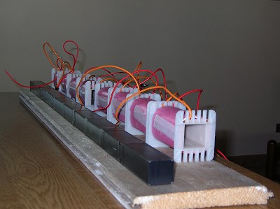
The winding will occupy 8 of the 10
ferrite blocks, leaving the two ends free. This is
useful since the value of µ-coil decreases as you move
away from the center of the bar. The two core elements
at the ends add to the total µ-coil but carry no
windings. In addition, the winding must not be done in a
single layer. It must be broken into sections: this
helps to decrease the parasitic capacitance by raising
the self resonance frequency.
SOME TECHNICAL DETAILS AND FINAL VALUES
Ferrite blocks are readily available
worldwide from large distributors of electronic
components such as RS-Components. The cost of each
ferrite block is approximately € 20.00. The blocks are
assembled together using a bicomponent glue. The joints
are reinforced with high strength adhesive tape, in a
longitudinal direction at each joint and along the
entire length of the bar. It is necessary to be careful
at this stage. The built bar is very delicate and can
easily break. The ferrite material is very brittle and
if it breaks, or falls, it splits into a thousand
crumbs, as if it were made of glass.
 |
 |
To build the winding we have approached manufacturers of transformers: and they have wound 8 spools with 12.000 turns each. They fit perfectly with the ferrite cores and give to the construction a very professional end result. Each winding is wrapped approximately with 0,33 kg of copper wire (2,5 kg for the entire induction coil) and the cost realized in this way is Euro 55,00 each section for a total of Euro 650,00 (10 ferrite blocks + 8 wound sections).
And these are the final values of the coil, measured with a HP 4274A RCL bridge, an oscilloscope, a function generator, a decade resistor box and a transmitting loop:
- Inductance coreless (without ferrite bar): 23 H @ 200 Hz with Q value of 2
- Inductance with ferrite core: 1650 H
- Resistance: 11220 Ohm
- Lower cut off frequency: 1,3 Hz
- Self resonating frequency: 200 Hz
- Parasite Capacitance: 385 pF (calculated)
- Thermal noise: 13,4 nV (calculated)
- µ-Rod (voltage output increasing): 158 (44 dB )
- µ-Coil (inductance increasing): 71 (Inductance with ferrite core/Inductance coreless), corresponding to 37 dB
The impedance of the coil just built
is very high and varies with frequency:
- 100 Hz = 1,43 MOhm (inductive)
- 50 Hz = 722 kOhm (inductive)
- 25 Hz = 355 kOhm (inductive)
- 10 Hz = 138 kOhm (inductive)
- 5 Hz = 65,9 kOhm (inductive)
- 2,5 Hz = 29,7 kOhm (inductive)
- 1 Hz = 13,1 kOhm (resistive)
- 0,5 Hz = 11,8 kOhm (resistive)
- 0,27 Hz = 11,3 kOhm (resistive)
- DC = 11,3 kOhm (resistive)
THE SHIELD
With such high values of impedance
the assembly of a shield is not just a possibility but
is a necessity. If the induction coil is not shielded it
will be sensitive to the electric field and the quality
of the reception will be compromised. We can use a grid
of thin metal to shield the sensor, like the one used to
make anti-mosquito grid for windows. This material is
readily available at hardware stores.
 |
 |
Before being installed the grid must be isolated: I got the insulation by mounting the moschito grid inside of two larger sheets of nylon bubble. The isolation is necessary because it is essential to make sure that the ends of the metallic net are not touching. Otherwise they form a single loop, a net metallic tube, that would work as short-circuit loop, lowering the sensitivity of the coil. The shield must cover the entire object, windings and ferrite bar: with high impedances ferrite rod is coupled capacitively to the windings becoming itself an electric field sensor. If you do not believe it try to to touch the ferrite with a finger: you will see the hum noise output from the coil to increase immediately, as if you were touching an oscilloscope probe.
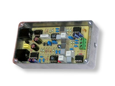
Choosing the circuit configuration and components
Here is the
schematic of the preamplifier used with our coil:
 |
Click here to see the scheme
in full resolution
a) The
Front-end:
The first stage design is very
important for the final result of the coil: it is very
easy to lose tens of dB in signal /noise ratio if this
stage is not optimised. We have chosen a balanced type
configuration with a virtual short circuit: we
tried different configurations, but this is the
one that gave the highest immunity to pick-up of the
electric field. It is very important because the
impedance of the coil is very high, so it is very likely
that the electric field together with the magnetic field
is received. To avoid this in addition to screening with
the grid we have chosen this type of configuration: the
electric field signals arrive in a common mode to the
amplifier and are then rejected. The coil works then in
current mode.
The gain of the first stage has been
chosen to be about 55 dB below 1 Hz, 12 dB at 100 Hz and
reaching the unity gain at 400 Hz : it is determined by
the ratio R1 + R2 resistors and the coil
impedance. This ensures that the entire operating range
from 0,1 to 100 Hz output overrides the input noise of
the operational noise input of the next stage. At the
same time it is not so high as to require offset
compensation and in any case is tolerated in terms
of product gain for bandwidth by the operational
amplifier.
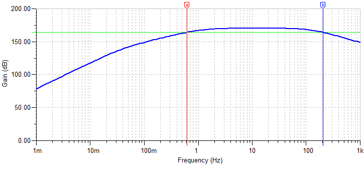 |
ICS101 Frequency response with LPF turned OFF: the device works in flat from 0.6 to 200 Hz (+/- 3 dB)
The choice of the operational amplifiers has been very laborious. The first selection was made based on values of voltage noise and current noise indicated in data-sheet, considering their effect on the coil impedance. The following amplifiers were taken into consideration: OP27, OP07, TL071, AD820, AD743, AD797, OP97 and LT1113. Unfortunately, many documents do not report data below 10 Hz. For a low noise performances in the available data sheet were the best the AD743 and OP07. Testing them we found that the first is better at 10 Hz, while the latter works better under 1 Hz. For this reason we decided to install in a first stage an OP07: choosing to give advantage in the coil performances to frequencies below 10 Hz.
Finally the capacity of 220 pF C8
introduces a low pass filter at about 220 Hz, to avoid
signals at higher frequencies saturating the stage
generating artifacts of measurement below 10 Hz. The low
frequency corner is instead determined by the inductance
of the coil and its intrinsic resistance: it is a low
pass filter at 1,3 Hz. A second pole is given by the
output capacitor of the amplifier circuit. However, they
are not a problem because under 1 Hz natural radio
signals grow in intensity: this compensates for loss of
sensitivity, giving a quasi-flat response.
b) The
low pass filter
It can be very useful, especially in
environments where 50 or 60 Hz are very intense, to
ensure that the natural background and the highest level
of hum noise are both included in the dynamic range of
the sound card. Its main function is then to lower
the level of hum noise, leaving the lower frequencies to
pass undisturbed. For this reason the filter must be
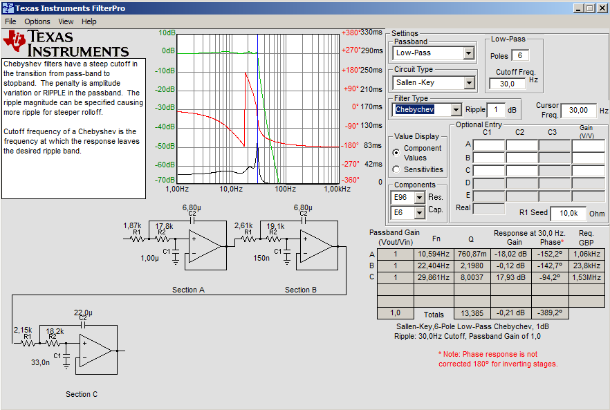
very steep and so we chose a 6 pole Chebychev
filter configuration : with it you have 44 dB of
attenuation at 50 Hz by placing the low frequency corner
to 30 Hz. Chebychev configuration was chosen
because the final low pass filter is steeper, even if it
shows a slight ripple on the frequency linearity. We
have chosen a Sallen-Key circuit because it uses fewer
parts and simpler. The design of the filter was
performed with the freeware software of Texas
Instruments "Filter Pro". Here below the screen
configuration with the end result.
 |
We rejected the idea of the notch
filter: difficult to produce and especially difficult to
maintain a stable frequency with changes in temperature
(do not forget that the coil operates usually outdoors,
with temperatures that can range from +40 ° C to - 30 °
C). The frequency of notch filter, especially if very
narrow and sharp, would be influenced by temperature.
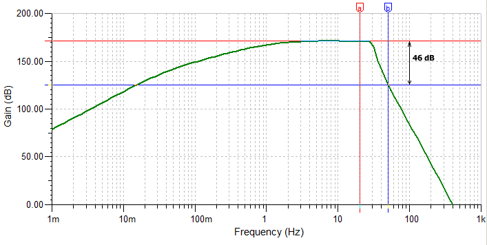 |
ICS101 Frequency response with LPF turned ON. At 50 Hz the attenuation is 46 dB
The 22 and 6,8 µF capacitors used in
the three sections of the filter must not be polarized.
This means that you need to use polyester capacitors
connected in parallel to reach the value shown. Do not
make compositions with electrolytic connected in phase
opposition: avoid these tricks. They do very strange
things deforming low frequency signals.
c) Final
amplifier
The final amplifier brings up the
signal level to ensure that it is strong enough for any
type of sound card. The goal of this amplifier is to
make sure that the input noise enters the first stage in
the dynamic window of the sound card: this way even the
slightest signal received by the coil will also be
displayed with your sound card.
There are three selectable gains: the
gain of 20 dB is usually the best and adapts to
mostlocations and sound cards. If once turned on the
coil the output signal exceeds 1 Vrms, you must
insert the low-pass filter or reduce the gain. The
maximum gain of 40 dB is recommended only in combination
with the low pass filter or with sound cards of low
gain.
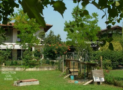
In my installation, where the coil is
placed in the garden 30 m away from home, the low pass
filter has been disabled and the gain is set to 20
dB.
d) Supply
stage
The power supply has two functions:
the first is to filter external power line disturbances.
Usually the most annoying noises are in the audio band:
the filtering is done with good results with
electrolytic capacitors. But very low frequency would
require very high values of the capacitor. Under these
conditions, an integrated circuit stabilizer gets better
results. An integrated circuit such as L7818 at 120 Hz
provides a separation of 60 dB, a value difficult to
achieve with electrolytic capacitors and resistors only
. For this reason an external 24 V supply was chosen to
ensure that the L7818 will filter the supply voltage
properly. The second function is to create a voltage
V/2, which will function as a virtual ground for input
stage and for the filter: it was simply made with a
common operational amplifier TL081C
Theoretical sensitivity
We now have all the data to estimate
the sensitivity of our coil thus constructed.
Let's take an example at 10 Hz.
We know that:
- Zcoil @ 10 Hz = 138 kOhm
- OP07 Vnoise @ 10 Hz = 10,3 nV in 1 Hz RBW (from OP07 data sheet)
- OP07 Inoise @ 10 Hz = 0,32 pA in 1 Hz RBW (from OP07 data sheet)
- Inoise flowing in Z coil will produces 44,36 nV (Inoise x Zcoil)
- Thermal noise of coil will be 14,42 nV (given by 11,3 kOhm wire resistance, Noise floor [nV/ sqrt Hz] = 4 x sqrt R [kohm])
- Total input noise @ 10 Hz = 47,77 nV (it will be the square sum of these three terms: OP07 Vnoise + Vnoise caused by Inoise flowing in Zcoil + Coil thermal noise)
Knowing the capturing area, it is
18.581 square meters, applying this formula:
E[v] = (4 x 3.14 x N x A x 6,28 x F x H) / 10.000.000 (http://www.vlf.it/minimal/minimal.htm)
we are now able to calculate the coil
sensitivity @ 10 Hz = 0,04 pT
Since on that frequency we expect
signal value of 0,3 pT we have a coil sensitivity of:
0,3 pT / 0,04 pT = 7,5
corresponding to a margin of 17,5 dB.
By the same calculations at other
frequencies we obtain:
@ 1 Hz, espected signal 1 pT,
coil sensitivity 0,2 pT, then a margin of 14 dB
@ 100 Hz, espected signal 0,1
pT, coil sensitivity 0,01 pT, then a margin of
20 dB
MEASURED SENSITIVITY: THE CHARACTERIZATION WITH A SOUND CARD
To make this measurement with the sound card we have to set the value of "equivalent noise bandwidth" to 1 Hz: it is different by the width of one FFT-bin. An example would be setting a sampling rate of 6000 S/s, 8192 FFT points and a "hamming" window of integration type. This will provide a value of 0,996 Hz equivalent noise bandwidth, suitable for our measure. You can also choose other settings to get this final value: SpectrumLab shows this value in the section "Configuration and display control / FFT proprieties".
Now we have to measure the background noise of our acquisition device (soundcard). To do this, once the coil is positioned far from house and connected to a PC by a coaxial line we turn (ON) off the power: the spectrum we detect is related to the input noise floor of our soundcard and all the noise coming from transmission lines we use to carry the signal from coil in the gardento the PC in the house.
Now we need to measure the noise of the preamplifier, but it varies with frequency because the inductor is not linear and varies its impedance: it changes so the value of noise generated by the current noise of the IC and changes the value of the operational amplifier gain. We need to realize therefore three resistance of 13,1 kOhm, 138 kOhm and 1,43 MOhm: these simulate the impedance of the coil at frequencies of 1, 10 and 100 Hz. We connect these resistors, instead of the coil, one by one, switching on the preamplifier with gain set to 20 dB and each time we read the values of noise in FFT curve at 1, 10 and 100 Hz. These three points will give the noise floor of our amplifier when it is fed by the coil. We can also do this for others but these three points are sufficient for an overview. With these three points we draw a curve that is the noise floor of our preamplifier.
Now we connect the preamplifier to
the coil and test the strength of received signals. They
must be at least 15 dB above the noise curve traced
before. If we achieve this result our device is
sensitive enough. But to know "how much" it is we have
yet to make a test: transmitting a known signal
strength. To do this I built a transmitting loop with 40
turns of diameter 45 cm.
 |
 |
The loop was placed 4.5 m from the coil, at 1.9 m height. In series is with the loop is a 1000 Ohm resistance connected to a function generator. After that signals are transmitted at various frequencies a floating oscilloscopeis used to measure the voltage across the resistance to then obtaining the current flowing in the loop. With this information, applying the law of Biot Savart we can calculate the field generated by our loop at a certain distance.
If you are unfamiliar with the
formula you can use the service of a websites like
this:
https://tiggerntatie.github.io/emagnet/offaxis/iloopcalculator.htm
Calculator for Off-Axis Fields Due to a Current Loop, by
Eric Dennison.
Applying the same signal strength for
all frequencies, and measuring a voltage of 3,66 V, then
3,66 mA of current, we have generated a field of 31 pT
on the coil. This signal is much stronger than natural
ones present and then we see them rise during normal
reception. The graph below sums this up:
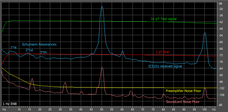 |
As we can see the sensitivity
obtained is very similar to that calculated and
at some frequencies even better: the gap between
the noise floor (yellow line) and the received signal
(blue line) is always maintained above 15 dB. A second
graph was made focusing on the lower part of the
spectrum: the most critical part being below 3 Hz.
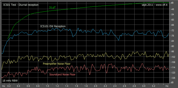 |
Here too the results are very good: our device is quite capable of receiving the geomagnetic pulsations. With these measures we are now able to evaluate the quality of our construction by comparing it to the specifications of a professional product used for research. We chose the model of MGC-3 Meda: it is a tool used by many research centers and reported on many academic papers.
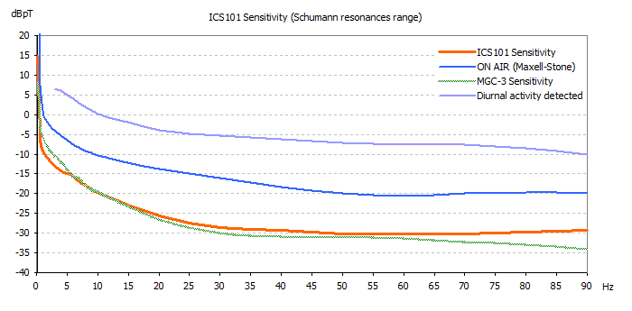
Here is the chart that compares the
characteristics in the region of Schumann resonances.
Two references were taken: the minimum signals detected
by Maxell / Stone in their famous paper and signals
detected in the daytime in our monitoring station, which
obviously are stronger. The graph shows the signals
expressed in dBpT: 0 dBpT correspond to 1 pT, 20 dBpT to
10 pT, -20 dBpT to 0,1 pT and so on.
 |
In this second picture we see how our
coils behave in the most difficult region of
geomagnetic pulsations frequencies, under 6 Hz.
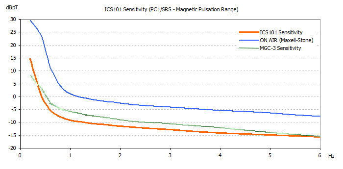 |
The measurements can be affected by some error: do not forget what we have done with the help of a single sound card, but, it appears clear that the device we constructed has characteristics very similar and comparable to a professional product. We can be very satisfied with this. Even the values of sensitivity that we calculated in the previous section are quite satisfied:
- At 1 Hz measured 0,34 pT, calculated was 0,2 pT
- At 10 Hz measured 0,07 pT, calculated was 0,04 pT
- At 100 Hz measured 0,03 pT, calculated was 0,01 pT
- 1 pT field gives a voltage output of 0,354 mV (+/- 3 dB)
- 1 mV voltage output corresponds to a field of 2,82 pT (+/- 3 dB)
Final results: what can we really get with this coil?
The initial goal was to build an
induction coil able to receive the Schumann Resonances
and geomagnetic pulsations with a soundcard: let us see
how it has been observed. .
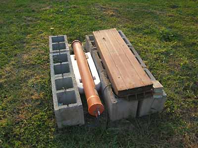 |
The coil, as described
above, was placed in the garden, 30 meters away
from the house and power lines, and positioned
to receive the North-South direction. The low
pass filter, after the characterization, has
been activated and the gain set to 20 dB. The
output signal from the coil was directly
connected to the LINE input of a standard type
Creative sound card.
The coil was immobilized with the hard foam packing between some cement blocks. This reduces the transmission of vibration of the soil by limiting the effect of microphonics. The coil is then covered to prevent falling rain from producing the same effect. |
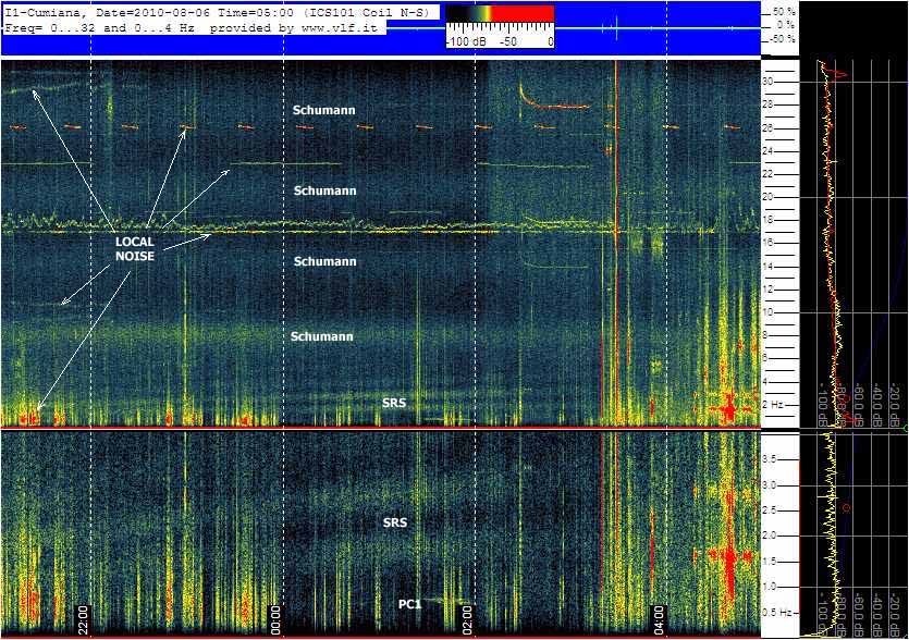
Example 1
4 hours of NS reception during the
2011 summer. Acquiring software SpectrumLab, analyzing
software: Sonic Visualizer.
 |
Here we can se a good PC1 geomagnetic
pulsation. It extends from 0,8 to 1,2 Hz and it emerges
from the background noise some times by more than 15 dB.
Schumann resonances are also clearly visible. Our coil
is doing a good job!
Example
2:
6 hours of NS reception during the
2011 summer. Acquiring software SpectrumLab, analyzing
software: Sonic Visualizer.
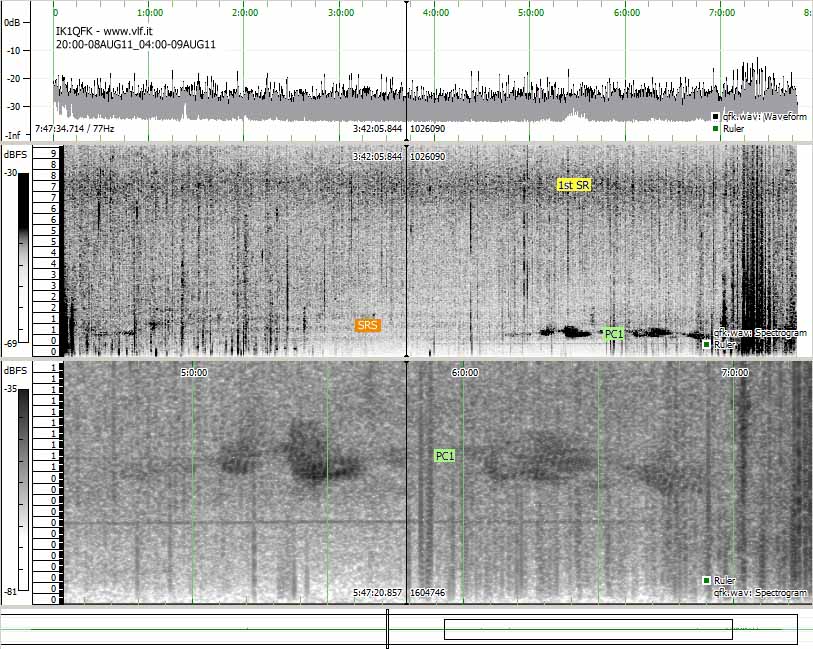 |
Here too we have received a
geomagnetic pulsations of type 1, even stronger than
before. Note that the pulse has the typical vertical
stripes that identify in an unequivocal way this type of
signal. But here we have another type of signal, a guest
more difficult to receive: a spectral resonaces
structure (SRS). It looks similar to the Schumann
resonance but with frequencies less than 3 Hz and with a
spacing of about 0,2 Hz
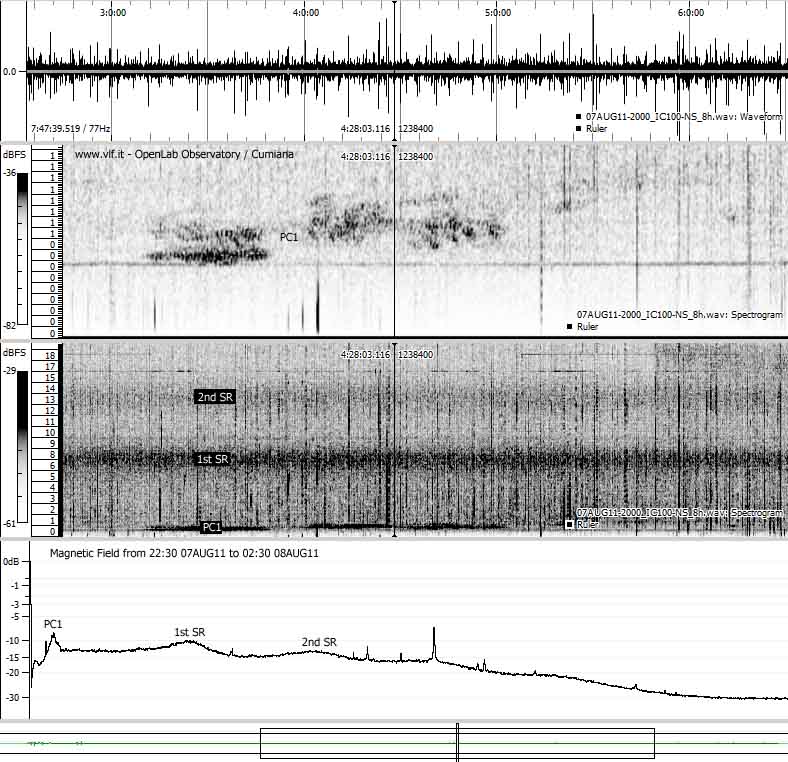
Example
3:
8 hours of NS reception during the
2010 summer. Acquiring software SpectrumLab, analyzing
software: SpectrumLab with unattended programmed
grabber.
 |
The signal SRS is much stronger than
in the previous example. According to a lot of
documentation that is available on the web they would be
due to the fluctuation of the magnetospheric tail under
the influence of the solar wind. They would be a direct
consequence of the Alfven resonance. Also are visible in
the spectrogram Schumann resonances and a weak PC1
pulsation. Our coil works just fine!
In the spectrogram are also present
many non-natural signals. They come from the power
supply in my house and by a high voltage power line just
1 km away from here. They unfortunately are not
excludable with the low-pass filter because are
located at lower frequency. The only way to avoid them
is to find a place sufficiently free from low frequency
electromagnetic pollution.
Beware of false signals
The position of the coil is very important: it should be situated away from power lines and devices that work on alternating current. A house in the countryside can be a good site but this is not always true: the power lines can disturb the reception even several miles away. A place in town is certainly a very critical position with little chance of success for good reception. Many signals we receive may not be natural but have the following origins:
a) Microphone effect. The coil also functions as a microphone: it hears the footsteps, the passage of vehicles and thunder. A geophone positioned near the coil can help to distinguish true signals from false signals.
b) The disturbance of the earth's magnetic field. It can be disrupted by any ferromagnetic metal object that moves close to the coil: just a bunch of keys to rotate a few feet away, and their track appears on the In the spectrogram. This also means that the coil must not be near where the metal parts that can vibrate, like fences or iron gates. Even the passage of cars causes of changes in the magnetic field within ten meters away.
c) Local sources. The coil should be located away from local ELF sources, such as: electric motors, pumps, washing machines, generators, charge controllers for solar panels, tube lamps, dimmer, CRTs,TVs, computers and any type of switching power supply.
d) Main power interharmonics (or Main power AM modulation) : Many signals arrive from the power supply: they are caused by non-linear loads that modulate in amplitude the network current. Many of these signals appear just like an AM modulation: for example you can see signals similar to PC1 at 1,5 Hz but are also present to 98,5 to 101,5 Hz. They are certainly not geomagnetic pulsations. To discover they sometimes need to run several spectrograms of the same signal at different FFT resolutions: this allows you to highlight details and find which are false signals. See for example the page of the observatory of Cumiana (http://www.vlf.it/cumiana/livedata.html) where the region of frequencies below 30 Hz is examined simultaneously in different ways: at high resolution with slow scrolling and with faster scrolling in multistrip graph.
Conclusions
There we have done it: we have built an induction coil with professional specifications, using as acquisition device a simple sound card. Now we too can receive similar geomagnetic pulsations such as HAARP .
Many Thanks to: Claudio Re for support during testing, advices and project documentation, Marco Bruno for advices and equipment provided, Andrea Dell'Immagine for various suggestions and the idea to use rectangular ferrites, Dave Ewer for grammar correction.
 |
 |
References
Induction coil sensors—a review, by
Slawomir Tumanski
Land Induction Coil (LIC) 120 data
sheet, KMS Technologies - KJT Enterprises Inc.
MGC-3 AC Magnetic Field Sensor data
sheet, MEDA, Inc.
BF-4 Magnetic Field Induction Sensor
data sheets, Schlumberger, EMI Technology Center
Ferrite rod antennas for HF? R.H.M.
Poole, BBC Research & Development
Return to vlf.it index